\( \newcommand{\vw}{\mathbf{w}} \newcommand{\vx}{\mathbf{x}} \newcommand{\vt}{\mathbf{t}} \newcommand{\vy}{\mathbf{y}} \newcommand{\vz}{\mathbf{z}} \newcommand{\vq}{\mathbf{q}} \newcommand{\vk}{\mathbf{k}} \newcommand{\vv}{\mathbf{v}} \newcommand{\vc}{\mathbf{c}} \newcommand{\vp}{\mathbf{p}} \newcommand{\vh}{\mathbf{h}} \newcommand{\vmu}{\boldsymbol{\mu}} \newcommand{\vsigma}{\boldsymbol{\sigma}} \newcommand{\vepsilon}{\boldsymbol{\epsilon}} \newcommand{\R}{\mathbb{R}} \newcommand{\E}{\mathbb{E}} \newcommand{\norm}[1]{\lVert #1 \rVert} \newcommand{\given}{\,\vert\,} \)

Lecture 17 — Architectural Building Blocks

Deep Learning · Advanced / Bonus

Kasemsit Teeyapan

Department of Computer Engineering, Chiang Mai University

Today

  1. The mindset: differentiable programming — if it’s differentiable, backprop learns it (L7)
  2. Embeddings for discrete & tabular data
  3. Differentiable discretization — soft binning, Gumbel-softmax, straight-through
  4. Conditioning (FiLM) and multi-task learning
  5. Mixture of Experts — conditional computation; scale parameters without scaling compute

This is an applied capstone: composing the primitives from L0L16 into new architectures. Paper-based.

The mindset: differentiable programming

A neural network is just a differentiable function built from differentiable parts. To invent a model:

  1. express your idea as a computation
  2. make every step differentiable (or relax it until it is)
  3. let backprop (L7) + SGD (L6) learn the parameters end-to-end

Pillar: the “layers” you know (conv, attention, norm) are just useful differentiable building blocks. You are free to design your own — the only rule is that gradients must flow.

Block 1: embeddings for discrete data

Categorical inputs (user id, product, zip code) → learned vectors, not one-hot.

  • a lookup table \(\mathbf{E}\in\R^{V\times D}\), trained with the model (L13)
  • learns similarity: related categories land nearby
  • entity embeddings beat one-hot on tabular data

One-hot = “everything is equally different.” An embedding learns the geometry — the same trick that powers word vectors (L13) and recommenders.

Block 2: differentiable discretization

Need a discrete choice (a bin, a category, a hard decision) but discreteness kills gradients. Relax it:

  • soft binning — softmax over bin centers → a soft one-hot
  • Gumbel-softmax — sample a category, differentiably
  • straight-through — hard forward, soft backward

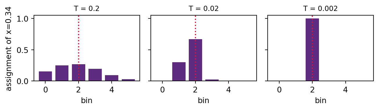
A temperature \(T\) interpolates soft ↔︎ hard.

\[\text{bin}_k(x) = \frac{\exp(-(x-c_k)^2/T)}{\sum_j \exp(-(x-c_j)^2/T)}\]

\(T\to 0\) recovers a hard bin — but for \(T>0\) it is differentiable.

Demo: soft → hard binning

import numpy as np, matplotlib.pyplot as plt
centers = np.linspace(0, 1, 6); x = 0.34
def soft_bin(x, T):
    z = -(x - centers)**2 / T; e = np.exp(z - z.max()); return e / e.sum()

fig, ax = plt.subplots(1, 3, figsize=(7.0, 2.1), sharey=True)
for a, T in zip(ax, [0.2, 0.02, 0.002]):
    a.bar(range(6), soft_bin(x, T), color="#5d2c80")
    a.set_title(f"T = {T}", fontsize=9); a.set_xlabel("bin"); a.axvline(2, color="crimson", ls=":")
ax[0].set_ylabel(f"assignment of x={x}")
plt.tight_layout(); plt.show()

The relaxation toolbox

Soft binning is one member of a big family: replace a hard operation with a temperature-controlled smooth surrogate so gradients flow.

  • soft-argmax → differentiable position (keypoints, pose)
  • softmax / attention (L10) = differentiable lookup / selection
  • Gumbel-softmax = differentiable sampling of a category
  • reparameterization (L12) = differentiable sampling of a continuous variable
  • NeuralSort / SoftSort → differentiable sorting & top-k
  • Sinkhorn / optimal transport → differentiable matching & permutations
  • soft-DTW → differentiable sequence alignment
  • perturbed optimizers → differentiate through an argmax / solver

Pillar: whenever a step is discrete, combinatorial, or “pick the best,” there is usually a soft, differentiable version. Reach for it, then anneal the temperature toward hard.

Block 3: conditioning with FiLM

Let one input modulate the processing of another. FiLM = feature-wise linear modulation:

\[\text{FiLM}(\vh) = \boldsymbol{\gamma}(\vc)\odot \vh + \boldsymbol{\beta}(\vc)\]

  • a side network maps condition \(\vc\) → scale \(\boldsymbol{\gamma}\), shift \(\boldsymbol{\beta}\)
  • cheap, powerful: used in style transfer, text-to-image (L12 guidance), VQA
  • cross-attention (L10) is the heavier cousin

Conditioning answers “do X, given Y” — the building block behind controllable and multimodal models.

Block 4: multi-task learning

One shared trunk, several task heads — learn related tasks together:

  • shared representation → better generalization (L4), less data per task
  • auxiliary tasks regularize the main one (L8)
  • watch for negative transfer & gradient conflict
  • balance losses by uncertainty weighting (Kendall 2018)

\[\mathcal L = \sum_t \frac{1}{2\sigma_t^2}\mathcal L_t + \log\sigma_t\]

Learn each task’s noise \(\sigma_t\) → the model down-weights hard/noisy tasks automatically.

Block 5: Mixture of Experts

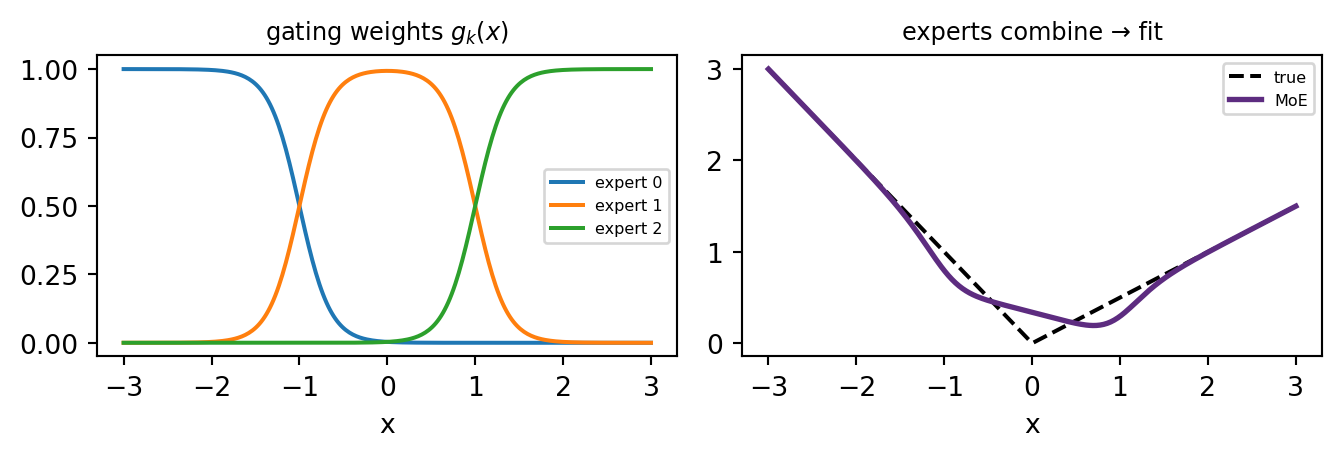
Instead of one big network, use many expert sub-networks + a gating network that routes each input:

\[\vy = \sum_{k=1}^{K} g_k(\vx)\, f_k(\vx), \qquad \textstyle\sum_k g_k = 1\]

  • sparse top-\(k\) routing: each token uses only 1–2 experts
  • scale parameters without scaling compute (the L14 lever!)
  • needs load balancing so all experts get used

Conditional computation: Mixtral, Switch, DeepSeek are MoE — trillions of parameters, but only a slice runs per token.

Demo: routing & specialization

import numpy as np, matplotlib.pyplot as plt
x = np.linspace(-3, 3, 300); ytrue = np.where(x < 0, -x, 0.5*x)     # a kinked function
anchors = np.array([-2.0, 0.0, 2.0])
def gate(x, T=0.7):
    z = -(x[:,None]-anchors[None])**2 / T; e = np.exp(z - z.max(1,keepdims=True)); return e/e.sum(1,keepdims=True)
G = gate(x); preds = np.zeros((len(x), 3))
for k in range(3):                                                   # each expert = gate-weighted linear fit
    w = G[:,k]; A = np.c_[x, np.ones_like(x)]
    c = np.linalg.lstsq(A*w[:,None], ytrue*w, rcond=None)[0]; preds[:,k] = A@c
mix = (G*preds).sum(1)

fig, ax = plt.subplots(1, 2, figsize=(7.0, 2.5))
for k in range(3): ax[0].plot(x, G[:,k], label=f"expert {k}")
ax[0].set_title("gating weights $g_k(x)$", fontsize=9); ax[0].legend(fontsize=6); ax[0].set_xlabel("x")
ax[1].plot(x, ytrue, "k--", label="true"); ax[1].plot(x, mix, color="#5d2c80", lw=2, label="MoE")
ax[1].set_title("experts combine → fit", fontsize=9); ax[1].legend(fontsize=6); ax[1].set_xlabel("x")
plt.tight_layout(); plt.show()
More blocks & the design loop

More primitives

  • inductive bias by construction — equivariance (L9), Deep Sets for permutation invariance
  • hypernetworks — a net that outputs another net’s weights
  • memory / retrieval — attend over an external store (RAG)

How to invent a model

  1. what’s the structure of my data? (encode it — L8/L9)
  2. what must be differentiable? (relax the rest)
  3. what should be shared vs conditional? (MTL / MoE)
  4. measure honestly (L4, L15) — did the bias help?

Summary

  1. Differentiable programming — design any computation; if gradients flow, you can learn it
  2. Embeddings turn discrete data into learnable geometry
  3. Differentiable discretization (soft binning / Gumbel-softmax) makes hard choices trainable
  4. FiLM conditions one signal on another; multi-task shares a trunk across tasks
  5. Mixture of Experts = conditional computation → more parameters, same compute (L14)

Something to think about: in a sparse MoE, routing is a discrete top-\(k\) choice. Which technique from this lecture lets you still train the gating network by gradient descent?

📌 Closing

You can now read the theory, run the demos, and compose the primitives into models that don’t exist yet.

That — not memorizing any one architecture — is what this course was for.

References: Guo & Berkhahn, Entity Embeddings (2016); Jang et al., Gumbel-Softmax (2017); Perez et al., FiLM (2018); Kendall et al., Multi-Task Uncertainty (2018); Shazeer et al., Sparsely-Gated MoE (2017); Fedus et al., Switch Transformer (2021); Zaheer et al., Deep Sets (2017).

⌂ Home