\( \newcommand{\vw}{\mathbf{w}} \newcommand{\vx}{\mathbf{x}} \newcommand{\vt}{\mathbf{t}} \newcommand{\vy}{\mathbf{y}} \newcommand{\vz}{\mathbf{z}} \newcommand{\vq}{\mathbf{q}} \newcommand{\vk}{\mathbf{k}} \newcommand{\vv}{\mathbf{v}} \newcommand{\vc}{\mathbf{c}} \newcommand{\vp}{\mathbf{p}} \newcommand{\vh}{\mathbf{h}} \newcommand{\vmu}{\boldsymbol{\mu}} \newcommand{\vsigma}{\boldsymbol{\sigma}} \newcommand{\vepsilon}{\boldsymbol{\epsilon}} \newcommand{\R}{\mathbb{R}} \newcommand{\E}{\mathbb{E}} \newcommand{\norm}[1]{\lVert #1 \rVert} \newcommand{\given}{\,\vert\,} \)

Lecture 10 — Attention & Transformers

Deep Learning · Session 10

Kasemsit Teeyapan

Department of Computer Engineering, Chiang Mai University

Today

  1. From hard-wired inductive bias (CNN) to learned relationships (attention)
  2. Self-attention = query–key–value, scaled dot-product
  3. Multi-head attention and the transformer layer (residual + norm, from L8)
  4. Positional encoding — putting order back in
  5. Decoder LMs (GPT), encoders (BERT), and the Vision Transformer

Reference: Bishop & Bishop (2024), Chapter 12Transformers

Recap → why attention?

  • L9: convolution bakes in locality — each unit sees a fixed small patch
  • But language needs long-range, content-based links:

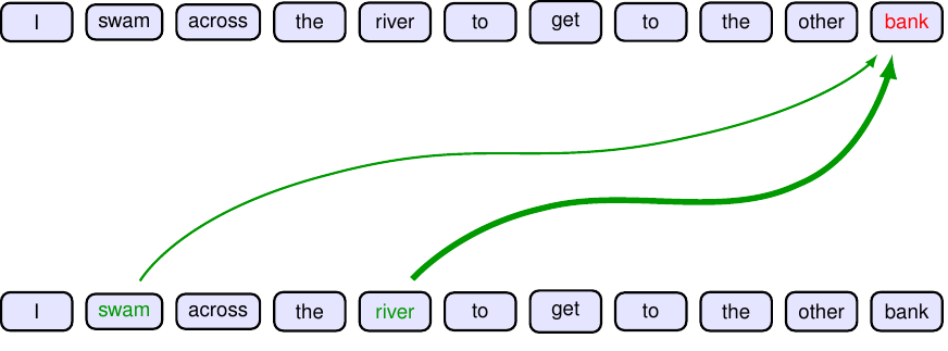
“…the bank of the river…”

“bank” depends on “river” — which could be anywhere in the sentence.

Source: Bishop & Bishop (2024), Fig 12.1 — meaning of “bank” resolved by attending to “river” / “swam”.

A CNN’s receptive field is fixed by architecture. We want connections that depend on the content, and that can reach any distance.

The idea: attention

Each token builds a query; every token offers a key and a value. A token’s output = a weighted average of values, weighted by query–key similarity.

  • Query \(\vq\) — “what am I looking for?”
  • Key \(\vk\) — “what do I offer?”
  • Value \(\vv\) — “what I pass on if matched”

Weights come from softmax of similarities → they sum to 1, and are data-dependent.

\[\text{Attention}(Q,K,V) = \text{softmax}\!\left(\frac{QK^\top}{\sqrt{d_k}}\right)V\]

The matrix \(QK^\top\) is every token scoring every token.

Self-attention: the dataflow

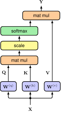
From one input matrix \(X\) (\(N\) tokens \(\times\, D\)):

\[Q = XW^{(q)},\;\; K = XW^{(k)},\;\; V = XW^{(v)}\]

  • “self” = Q, K, V all come from the same sequence
  • the learnable parts are only \(W^{(q)}, W^{(k)}, W^{(v)}\)
  • output \(Y\) has the same shape as \(X\) → stackable

Source: Bishop & Bishop (2024), Fig 12.6 — scaled dot-product self-attention.

🔢 Worked example: attention by hand

Three tokens, \(d_k=2\). Query of token A: \(\vq=[1,1]\). Keys/values: \(\vk_A=[1,1],\,\vk_B=[1,-1],\,\vk_C=[-1,1]\); \(\;\vv_A=[1,0],\,\vv_B=[0,1],\,\vv_C=[1,1]\).

1. Scores \(\vq\cdot\vk_j\), then \(/\sqrt{d_k}=/\sqrt2\): \[[2,\,0,\,0]\;\to\;[1.41,\,0,\,0]\]

2. Softmax → attention weights: \[\frac{[e^{1.41},1,1]}{e^{1.41}+2}=[0.67,\,0.16,\,0.16]\]

3. Weighted sum of values: \[0.67\,\vv_A+0.16\,\vv_B+0.16\,\vv_C\] \[=[0.83,\;0.33]\]

Token A attends mostly to itself (0.67) because its query matched its own key best → its output is mostly \(\vv_A\). That’s the whole mechanism — repeat per token.

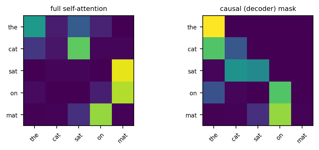
Demo: self-attention from scratch

import numpy as np, matplotlib.pyplot as plt
rng = np.random.default_rng(0)
tokens = ["the", "cat", "sat", "on", "mat"]
N, d = len(tokens), 16
X = rng.normal(size=(N, d))
Wq, Wk, Wv = (rng.normal(size=(d, d)) * 0.5 for _ in range(3))
Q, K, V = X @ Wq, X @ Wk, X @ Wv

def softmax(z):
    z = z - z.max(-1, keepdims=True); e = np.exp(z); return e / e.sum(-1, keepdims=True)

mask = np.triu(np.ones((N, N)), 1) * -1e9          # causal: no peeking ahead
A      = softmax(Q @ K.T / np.sqrt(d))             # full self-attention
A_caus = softmax(Q @ K.T / np.sqrt(d) + mask)      # decoder (masked)

fig, ax = plt.subplots(1, 2, figsize=(6.2, 2.6))
for a, M, t in zip(ax, [A, A_caus], ["full self-attention", "causal (decoder) mask"]):
    a.imshow(M, cmap="viridis", vmin=0, vmax=1)
    a.set_xticks(range(N)); a.set_xticklabels(tokens, fontsize=7, rotation=45)
    a.set_yticks(range(N)); a.set_yticklabels(tokens, fontsize=7); a.set_title(t, fontsize=8)
plt.tight_layout(); plt.show()
Why scale by √dₖ ?

\(\vq\cdot\vk = \sum_{i=1}^{d_k} q_i k_i\). If entries are \(\sim\!\mathcal N(0,1)\), the dot product has variance \(\approx d_k\).

  • large \(d_k\) → large logits → softmax saturates → gradients vanish (L7!)
  • dividing by \(\sqrt{d_k}\) keeps variance \(\approx 1\)

Pillar: the \(\sqrt{d_k}\) is not cosmetic — without it, attention collapses to a hard max early in training and stops learning.

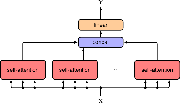
Multi-head attention

One attention = one way of relating tokens. Run \(h\) of them in parallel, each with its own \(W^{(q)},W^{(k)},W^{(v)}\), then concat → linear.

  • different heads learn different relations (syntax, coreference, position…)
  • like multiple filters in a CNN (L9), but for relations

Source: Bishop & Bishop (2024), Fig 12.8 — heads run in parallel, then concatenate.

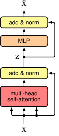
The transformer layer

A block = multi-head attention + a position-wise MLP, each wrapped in residual + layer-norm (L8!):

\[\begin{aligned} Z &= \text{LayerNorm}(X + \text{MHA}(X))\\ \tilde X &= \text{LayerNorm}(Z + \text{MLP}(Z))\end{aligned}\]

  • attention mixes tokens; MLP processes each token
  • residual + norm → train very deep stacks

Source: Bishop & Bishop (2024), Fig 12.9 — one transformer layer.

Positional encoding

Attention is permutation-equivariant — it has no idea of order! Shuffle the tokens, the output just shuffles too.

So we add position information to each embedding:

\[\tilde{\vx}_n = \vx_n + \vp_n\]

  • fixed sinusoids (original) or learned position vectors
  • order is now in the data, not the architecture

A CNN knows position from its grid. Attention sees a set. Without \(\vp_n\), “dog bites man” = “man bites dog”.

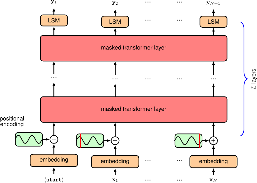
Putting it together: GPT

A decoder LM: embed tokens + positions → stack of masked transformer layers → linear-softmax → next-token distribution.

  • trained to predict the next token (self-supervised, L11 next)
  • causal mask → can’t see the future
  • generate by sampling, feeding output back in

Source: Bishop & Bishop (2024), Fig 12.15 — GPT decoder architecture.

Encoders, decoders, and vision

  • Decoder (GPT): causal mask, generates text
  • Encoder (BERT): no mask, sees whole sequence both ways → understanding tasks (Fig 12.18)
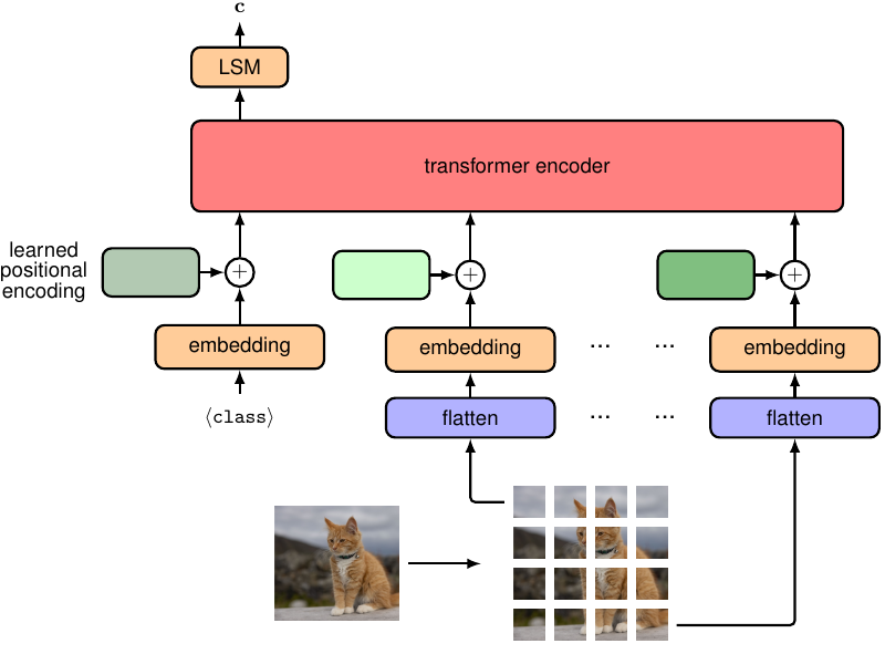
  • Vision Transformer: cut image into patches, treat as tokens → no convolution at all!

Source: Bishop & Bishop (2024), Fig 12.22 — Vision Transformer (ViT).

Full circle (L9): ViT throws away convolution’s built-in image bias and relearns it from data — viable only with large-scale pretraining (L13).

Complexity: the catch

\(QK^\top\) is \(N\times N\)\(O(N^2)\) in sequence length.

  • doubles the context → the compute & memory
  • the central engineering bottleneck of long-context LLMs
  • vs RNNs: \(O(N)\) but sequential (no parallelism, BPTT vanishing gradients)

Transformer trade: parallel + long-range, but quadratic in length.

This is why “context window” is a headline number — and a cost.

Summary

  1. Attention = content-based, data-dependent connections — softmax\((QK^\top/\sqrt{d_k})V\)
  2. Self-attention learns relations; only \(W^{(q)},W^{(k)},W^{(v)}\) are trained
  3. Multi-head + MLP + residual/norm (L8) = the transformer layer
  4. Positional encoding restores order; attention alone sees a set
  5. GPT / BERT / ViT — one architecture, swap the mask & the data; cost is \(O(N^2)\)

Something to think about: in a decoder, why apply the causal mask before the softmax (as \(-\infty\)) rather than zeroing weights after? (Hint: what must each row still sum to?)

📌 Read before next class

Representation Learning & Self-Supervised Learning

Autoencoders, and contrastive learning (SimCLR) — how to learn useful representations without labels, the engine behind modern pretraining.

Reading: Chen et al., A Simple Framework for Contrastive Learning (SimCLR) (2020). Figures from Bishop & Bishop (2024), Ch 12 — https://www.bishopbook.com/. References: Vaswani et al., Attention Is All You Need (2017); Dosovitskiy et al., ViT (2021); Devlin et al., BERT (2019).

⌂ Home