\( \newcommand{\vw}{\mathbf{w}} \newcommand{\vx}{\mathbf{x}} \newcommand{\vt}{\mathbf{t}} \newcommand{\vy}{\mathbf{y}} \newcommand{\vz}{\mathbf{z}} \newcommand{\vq}{\mathbf{q}} \newcommand{\vk}{\mathbf{k}} \newcommand{\vv}{\mathbf{v}} \newcommand{\vc}{\mathbf{c}} \newcommand{\vp}{\mathbf{p}} \newcommand{\vh}{\mathbf{h}} \newcommand{\vmu}{\boldsymbol{\mu}} \newcommand{\vsigma}{\boldsymbol{\sigma}} \newcommand{\vepsilon}{\boldsymbol{\epsilon}} \newcommand{\R}{\mathbb{R}} \newcommand{\E}{\mathbb{E}} \newcommand{\norm}[1]{\lVert #1 \rVert} \newcommand{\given}{\,\vert\,} \)

Lecture 14 — Scaling & Modern AI Systems

Deep Learning · Session 14

Kasemsit Teeyapan

Department of Computer Engineering, Chiang Mai University

Today

  1. The Bitter Lesson — general methods + compute beat hand-crafted knowledge
  2. Scaling laws — loss falls as a power law in parameters, data, compute
  3. Compute-optimal training — Kaplan vs Chinchilla (~20 tokens/parameter)
  4. Emergent abilities — and an honest caveat about how we measure them
  5. Foundation models, and the limits: data, energy, cost

Sources: Kaplan et al. (2020); Hoffmann et al. (2022); Wei et al. (2022). Bishop §12.3.5 frames this but contains no scaling laws — this lecture is paper-based.

Recap → the question

  • L0: success came from data + compute + algorithms
  • L11: self-supervised pretraining unlocks all data
  • L13: in-context learning is emergent at scale

Now we make this quantitative.

Is “make it bigger” just folklore — or is there a law? If we double compute, can we predict the gain before spending millions of dollars training?

The Bitter Lesson

“The biggest lesson… is that general methods that leverage computation are ultimately the most effective.” — Sutton, 2019

  • 70 years of AI: hand-built knowledge loses to learning + search + scale
  • chess, Go, vision, speech, language — same story each time

Pillar: the inductive biases we lovingly engineer (L8/L9) help at small scale, but at large scale, data + compute + a general architecture win.

Scaling laws

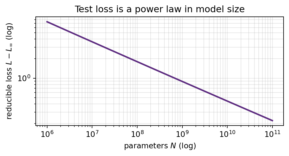
Kaplan et al. (2020): test loss is a power law in each of model size \(N\), data \(D\), and compute \(C\) — over many orders of magnitude:

\[L(N) \approx L_\infty + \left(\frac{N_c}{N}\right)^{\alpha}\]

  • straight line on a log-log plot
  • smooth, predictable — no sign of the classical overfitting wall (L4!)

You can fit the curve on small models and extrapolate to predict the loss of a model too expensive to train.

Demo: the power law

import numpy as np, matplotlib.pyplot as plt
E, A, B, a, b = 1.69, 406.4, 410.7, 0.34, 0.28      # Chinchilla-form constants
N = np.logspace(6, 11, 60)
L = E + A/N**a + B/(20*N)**b                          # ample data (~20 tokens/param)

plt.figure(figsize=(5.4, 3.0))
plt.loglog(N, L - E, lw=2, color="#5d2c80")
plt.xlabel("parameters $N$ (log)"); plt.ylabel("reducible loss $L-L_\\infty$ (log)")
plt.title("Test loss is a power law in model size"); plt.grid(True, which="both", alpha=0.3)
plt.tight_layout(); plt.show()

Compute-optimal: Kaplan vs Chinchilla

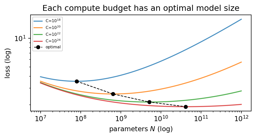
Fixed compute budget \(C \approx 6ND\). Spend it on a bigger model or more data?

  • Kaplan (2020): mostly grow \(N\) (models)
  • Chinchilla (2022): earlier LLMs were undertrained — scale \(N\) and \(D\) together, roughly ~20 tokens per parameter

Chinchilla (70B) beat Gopher (280B) using a 4× smaller model trained on more data — same compute.

Demo: the compute-optimal frontier

import numpy as np, matplotlib.pyplot as plt
E, A, B, a, b = 1.69, 406.4, 410.7, 0.34, 0.28
plt.figure(figsize=(5.4, 3.0))
opt_N, opt_L = [], []
for C in [1e18, 1e20, 1e22, 1e24]:
    N = np.logspace(7, 12, 300); D = C/(6*N)         # fixed compute: C = 6ND
    L = E + A/N**a + B/D**b
    plt.loglog(N, L, alpha=0.8, label=f"C=10$^{{{int(np.log10(C))}}}$")
    i = np.argmin(L); opt_N.append(N[i]); opt_L.append(L[i])
plt.loglog(opt_N, opt_L, "ko--", lw=1, ms=5, label="optimal")
plt.xlabel("parameters $N$ (log)"); plt.ylabel("loss (log)")
plt.title("Each compute budget has an optimal model size"); plt.legend(fontsize=6)
plt.tight_layout(); plt.show()
Emergent abilities

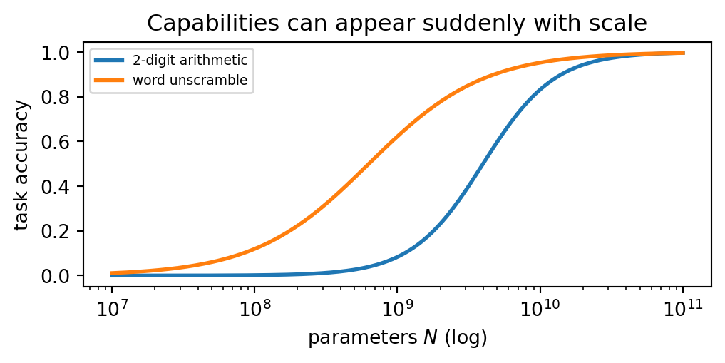
Wei et al. (2022): some abilities are near-random until a scale threshold, then jump sharply.

  • multi-step arithmetic, word unscrambling, in-context reasoning
  • not predicted by the smooth loss curve

Honest caveat (Schaeffer, 2023): some “emergence” is a measurement artifact — harsh metrics (exact match) hide smooth underlying gains. Always ask how it was measured.

Demo: an emergence curve

import numpy as np, matplotlib.pyplot as plt
logN = np.linspace(7, 11, 200)
sig = lambda x: 1/(1+np.exp(-x))
plt.figure(figsize=(5.4, 2.8))
for name, thr, w in [("2-digit arithmetic", 9.6, 0.25), ("word unscramble", 8.8, 0.4)]:
    plt.plot(10**logN, sig((logN-thr)/w), lw=2, label=name)
plt.xscale("log"); plt.xlabel("parameters $N$ (log)"); plt.ylabel("task accuracy")
plt.title("Capabilities can appear suddenly with scale"); plt.legend(fontsize=7)
plt.tight_layout(); plt.show()

Foundation models

Scale turns one pretrained model into a platform:

  • pretrain once at scale → adapt to thousands of tasks (L11 transfer)
  • the “new Moore’s law”: training compute doubling ~every 3.4 months since 2012 (Bishop §1.1, Fig 1.16)
  • GPT, Gemini, Claude, Llama — same recipe, more scale

Pillar: scaling is the empirical answer to L4’s question — with enough data and capacity, generalization keeps improving, guided by power laws rather than the classical bias–variance fear.

The limits of scale

  • data wall — we are running out of high-quality text
  • energy & cost — training runs cost tens of millions; large carbon footprint
  • inference cost — serving at scale dominates lifetime compute
  • concentration — only a few labs can afford frontier models

Scaling laws say bigger is better — but they say nothing about whether bigger is affordable, safe, or fair. That motivates L15L16.

Summary

  1. Bitter Lesson — general methods + compute beat hand-engineered knowledge
  2. Scaling laws — loss is a smooth power law in \(N\), \(D\), \(C\) (predictable, extrapolable)
  3. Compute-optimal — Chinchilla: scale data with parameters (~20 tokens/param)
  4. Emergent abilities appear with scale — but mind how they’re measured
  5. Foundation models = scale + transfer; limited by data, energy, cost

Something to think about: scaling laws are fit on today’s data and architectures. Name one reason the curve could bend — for better or worse — that the power law wouldn’t predict.

📌 Read before next class

Trustworthy AI — calibration & uncertainty

A model can be accurate and badly overconfident. How do we know when to trust a prediction?

Reading: Guo et al., On Calibration of Modern Neural Networks (2017). References: Kaplan et al. Scaling Laws (2020); Hoffmann et al. Chinchilla (2022); Wei et al. Emergent Abilities (2022); Schaeffer et al. Mirage? (2023); Sutton, The Bitter Lesson (2019).

⌂ Home