Lecture 0 — Introduction & The Deep Learning Revolution

Deep Learning · Session 0

Kasemsit Teeyapan

Department of Computer Engineering, Chiang Mai University

Today

What is this course about, and why focus on theory in an era when LLMs can write code for us?
How has Deep Learning transformed the world?
The central problem of the course: learning functions from data.
The very first example: polynomial curve fitting → introducing overfitting, generalization, and regularization.
Why does “deep” work so well?

Part 1 · About This Course

Theory?

LLMs can already write code to train models and explain theory remarkably well. They can answer:

Why is the loss not decreasing?
Why does a larger model sometimes generalize better?
Which architecture should I choose, and why?

And they are often correct.

So why do we still need to study the theory?

Because you must be the one who can…

Judge whether an answer is actually correct.
Ask the right questions.
Go beyond what the LLM already knows.

What AI does for you vs. what you must understand

What we used to spend time on…

TensorFlow / PyTorch syntax
library APIs
writing the training loop
calling the optimizer

What this course emphasizes

Why does Adam converge faster than SGD in some cases?
Why does batch norm make training easier?
Why can attention replace recurrence?

Code as a tool to make theory concrete.

Course roadmap

Before midterm

Mathematical foundations (probability, MLE)
Linear models; classification & decision theory
Statistical learning & generalization
Neural networks; backprop; optimization
Regularization
Convolutional networks

After midterm

Computer-vision tasks; Transformers & attention
Representation & self-supervised learning
Language models & scaling laws (LLMs)
Generative models (VAE, GAN, Diffusion)
Trustworthy AI; distribution shift & OOD
Maybe: EM, sampling, MoE, etc.

We read research papers

ํYou will read landmark papers, not just the textbook.

A few we will read:

Rumelhart et al. (1986) — backprop
Kingma & Ba (2015) — Adam
He et al. (2016) — ResNet
Vaswani et al. (2017) — Transformers
Ho et al. (2020) — diffusion (DDPM)
Hoffmann et al. (2022) — Chinchilla

How it works

Read the assigned paper before class
A short reading quiz in class every 2–3 weeks
We discuss it together (journal club)
One in-depth paper review during the term

Assessment

Component	Weight
Midterm exam (written)	35%
Final exam (written)	35%
Reading quizzes (in-class)	15%
Paper review (take-home)	15%

AI usage policy

✅ Allowed

Writing / debugging code
Asking AI to explain concepts you don’t get
The take-home paper review (briefly disclose how you used it)

Disclosure is for transparency, not for losing marks.

❌ Not allowed

During the midterm / final exam
During in-class reading quizzes

The one rule that matters: if you submit work you cannot explain, you don’t understand it yet — and the exams will reveal it.

Course information

Prerequisites

Calculus (basics)
Linear algebra (basics)
Probability (basics)
Programming in Python (Example codes)

Contact & resources

Instructor: Kasemsit Teeyapan
Email / office hours: kasemsit.t@cmu.ac.th + MS Teams
Textbook: Bishop (2024) — bishopbook.com
Slides & announcements: Mango Canvas

Part 2 · The Deep Learning Revolution

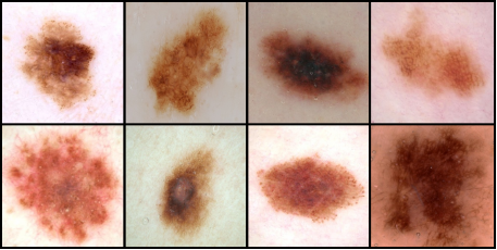
DL diagnoses skin cancer at expert level

Task: an image of a skin lesion → melanoma or not?
The model learns from hundreds of thousands of images with no hand-written rules for what cancer looks like
Accuracy on par with expert dermatologists

Key idea: the model learns the features that discriminate, directly from raw data

Bishop Fig 1.1 — dermoscopic images of skin lesions

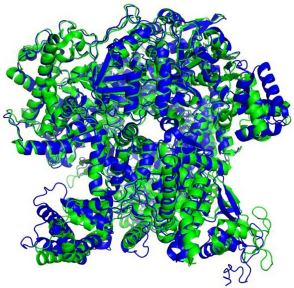
DL predicts protein structure (AlphaFold)

A 50-year-old open problem: amino-acid sequence → 3-D structure
AlphaFold predicts at near-experimental accuracy (green = predicted, blue = true)
It transformed all of structural biology

Same pattern: lots of data + a deep model + compute → solving problems we can’t write rules for

Generative AI: creating, not just classifying

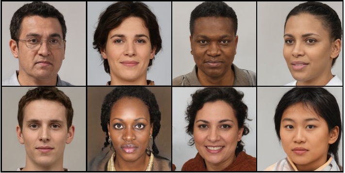
These faces are not real people — a deep network generated them
The same idea powers image generators (diffusion) and LLMs that write text and code
The model learns the distribution of data, then samples new examples

We will build up to this: VAEs, GANs, diffusion in the second half.

Source: Bishop & Bishop (2024), Deep Learning, Fig 1.3 — faces synthesized by a GAN

Superhuman game play: AlphaGo

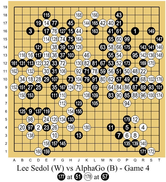
2016: AlphaGo beat Lee Sedol, a world champion, at Go
Go has more board positions than atoms in the universe — brute force is impossible
It learned strategy by self-play (reinforcement learning) + deep networks

Move 37 (game 2) was so creative that commentators thought it was a mistake — then it won.

Source: Wikimedia Commons — Lee Sedol vs AlphaGo, Game 4 by Wesalius, CC BY-SA 4.0

Conversational AI & code: large language models

ChatGPT, Gemini, Claude answer questions, write essays, and generate code
One model — trained only to predict the next word on internet-scale text — picks up grammar, facts, translation, and step-by-step reasoning
It is the tool that writes your boilerplate, and exactly why this course is theory-first: you must judge when its output is right

Same recipe again: a Transformer trained self-supervised at massive scale. The second half of the course shows how — and why “bigger” keeps working.

LLM/ChatGPT = แอปที่นักศึกษาทุกคนรู้จักและใช้จริง — ใส่เป็นตัวอย่างเด่น โมเดลเดียวเทรนด้วยงานง่าย ๆ “ทายคำถัดไป” บนข้อความระดับอินเทอร์เน็ต แต่ได้ไวยากรณ์/ความรู้/การแปล/การให้เหตุผลมาเป็นผลพลอยได้ เชื่อมปรัชญาวิชา: LLM เขียนโค้ดแทนได้ → เราจึงเน้นทฤษฎี เพื่อให้ “ตัดสินได้ว่าผลลัพธ์มันถูกเมื่อไหร่” ย้ำ recipe เดิม: Transformer + self-supervised + scale (ครึ่งหลังจะเจาะ) ~1.5 นาที

…and it’s already everywhere

🗣️ Speech recognition — voice assistants, dictation
🌐 Machine translation — Google Translate
🚗 Autonomous driving — perception from cameras/LiDAR

🎬 Recommendation — YouTube, Netflix, TikTok feeds
🌦️ Weather & science — GraphCast forecasting, drug discovery
🩺 Medical imaging — beyond melanoma: X-ray, retina, pathology

Wildly different domains, one toolkit: learn features from data, at scale. That toolkit is what this course takes apart.

สไลด์ montage ให้เห็น breadth: DL อยู่ในชีวิตประจำวันแล้ว — speech (ผู้ช่วยเสียง), แปลภาษา (Google Translate), รถยนต์ไร้คนขับ, ระบบแนะนำ (YouTube/Netflix/TikTok), พยากรณ์อากาศ/ค้นยา (GraphCast), ภาพการแพทย์ (X-ray/จอประสาทตา) ย้ำ takeaway: โดเมนต่างกันสุดขั้ว แต่ “กล่องเครื่องมือเดียวกัน” — เรียน feature จากข้อมูลที่สเกลใหญ่ ซึ่งเป็นสิ่งที่วิชานี้จะถอดประกอบ ~1.5 นาที

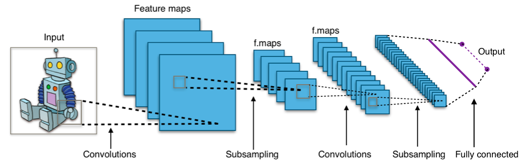
Representation learning: features in layers

Early layers learn simple features (edges, colors)
Deeper layers combine them into complex concepts (textures → parts → objects)
Nobody designs these features — they emerge from data

This learned hierarchy is what we mean by “deep”.

Source: Wikimedia Commons — Typical CNN by Aphex34, CC BY-SA 4.0

A Brief History — and Why Now

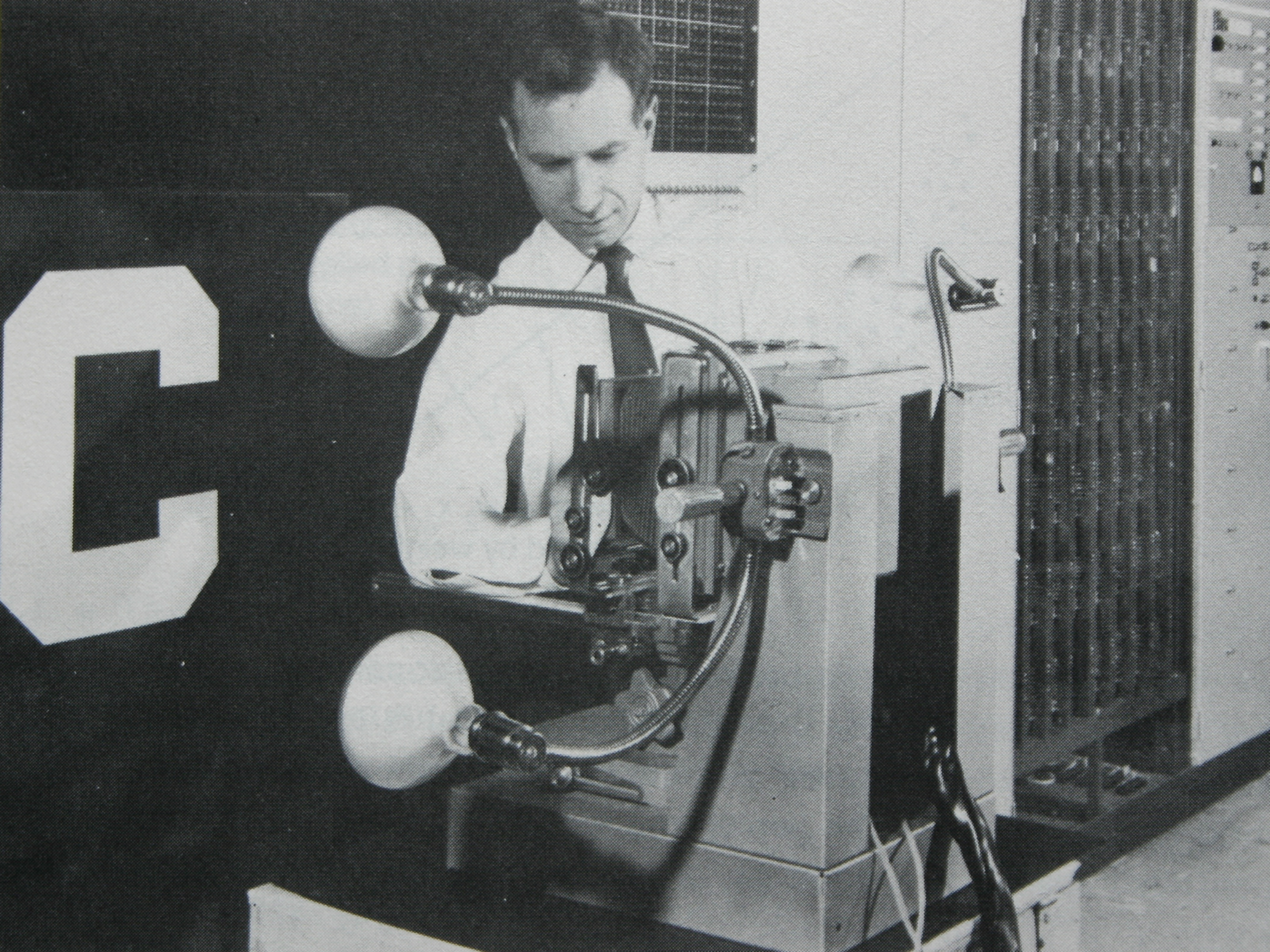
It started in 1958: the Perceptron

The ideas are old — what changed is scale.

1958 Rosenblatt’s Perceptron (the machine shown)
1986 Backpropagation popularized
2012 AlexNet wins ImageNet → the deep learning era begins
2017 Transformers (“Attention is all you need”)
2020s LLMs (GPT), diffusion models, AlphaFold

Source: Bishop & Bishop (2024), Deep Learning, Fig 1.14 — the Mark 1 Perceptron

Why now? Three drivers

Data — internet-scale labeled datasets (e.g. ImageNet)
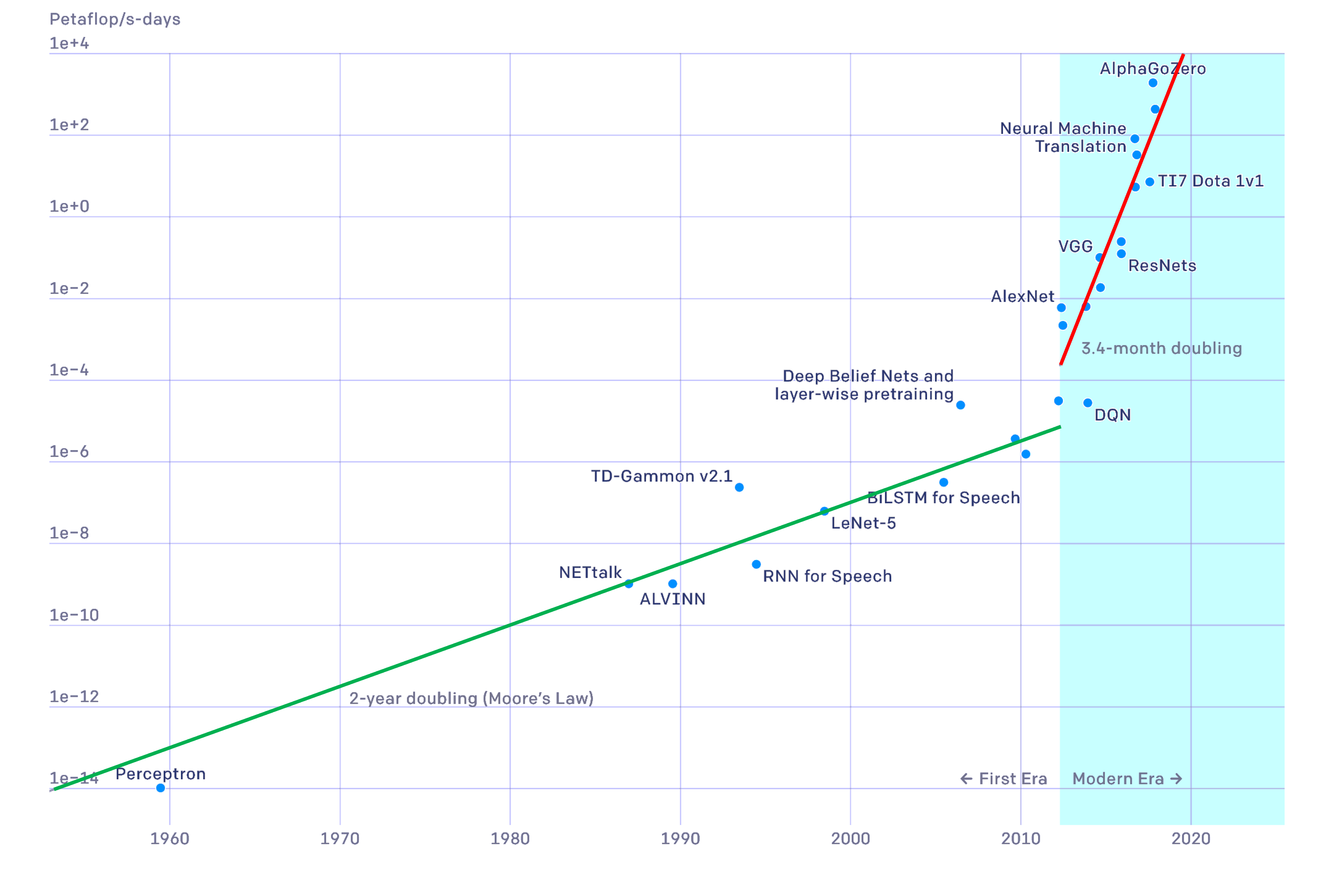
Compute — GPUs; training compute has exploded
Algorithms — ReLU, dropout, batch norm, attention

Same math as the 1980s — but \(10^{10}\times\) more compute.

Source: Bishop & Bishop (2024), Deep Learning, Fig 1.16 — training compute over time (note: log scale)

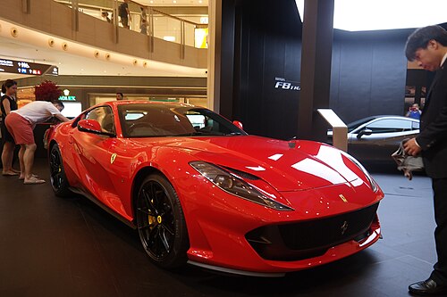
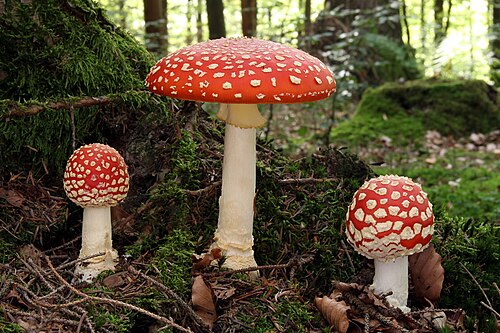
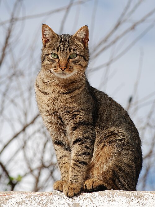
What is ImageNet?

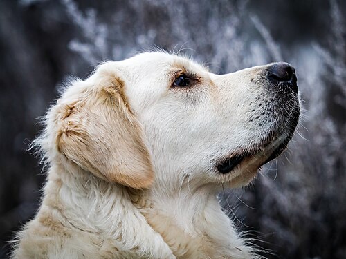
golden retriever

sports car

fly agaric

tabby cat

A huge hand-labeled image database (~14M images, ~20k categories) — Deng, …, Fei-Fei (2009)
The ILSVRC contest (2010–2017) used a 1000-category subset (~1.2M training images) — e.g. 120 dog breeds alone!
Task: put each image in 1 of 1000 classes, scored by top-5 error (correct if the true label is among the model’s top-5 guesses)

Example photos: Wikimedia Commons (CC BY / BY-SA) — retriever © Dietmar Rabich; cat © Alvesgaspar; Ferrari © David290; fly agaric © Holger Krisp

อธิบายว่า ImageNet คือฐานข้อมูลภาพที่มนุษย์ label ขนาดมหึมา (Fei-Fei Li 2009) และ ILSVRC คือ “การแข่งขัน” ประจำปีที่ใช้ subset 1000 คลาส ~1.2 ล้านภาพ ชี้รูป 4 ใบเป็นตัวอย่างคลาส เกร็ด: มีสุนัขถึง 120 สายพันธุ์ → คลาสละเอียดมาก อธิบาย top-5 error: ทายได้ 5 อันดับ ถ้ามีคำตอบจริงถือว่าถูก (เพราะบางภาพกำกวม) นี่คือสนามวัดความเก่ง สไลด์ถัดไปดูผลการแข่ง ~2 นาที

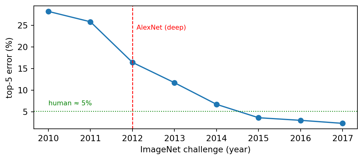
🔬 The 2012 turning point

import matplotlib.pyplot as plt
years = [2010, 2011, 2012, 2013, 2014, 2015, 2016, 2017]
err   = [28.2, 25.8, 16.4, 11.7, 6.7, 3.6, 3.0, 2.3]   # ILSVRC winning top-5 error (%)
plt.figure(figsize=(6.2, 2.8))
plt.plot(years, err, "o-")
plt.axvline(2012, color="r", ls="--", lw=1); plt.text(2012.1, 24, "AlexNet (deep)", color="r", fontsize=8)
plt.axhline(5.1, color="g", ls=":", lw=1);   plt.text(2010, 6.5, "human ≈ 5%", color="g", fontsize=8)
plt.xlabel("ImageNet challenge (year)"); plt.ylabel("top-5 error (%)"); plt.tight_layout(); plt.show()

In 2012 a deep network nearly halved the error overnight — and passed the human estimate by 2015.

Source: winning top-5 error, ILSVRC 2010–2017. Human ≈ 5.1% is A. Karpathy’s single-annotator estimate (blog, 2014), not an official number.

Part 3 · The Core Problem: Learning a Function from Data

Supervised learning

Given \(N\) training pairs \(\{(x_n, t_n)\}_{n=1}^{N}\) (input, target), find a function \(y(x)\) that predicts \(t\) — even on data it has never seen (generalization).

All of deep learning comes down to choosing the form of \(y(x,\vw)\) and how to adjust the parameters \(\vw\) from data.

Part 4 · A First Example: Polynomial Curve Fitting

A toy example that teaches the whole course

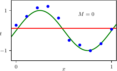
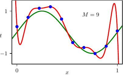
The true data come from \(\sin(2\pi x)\) (green) + noise
We only see the blue points — \(N\) of them — not the green curve
Goal: recover the underlying relationship

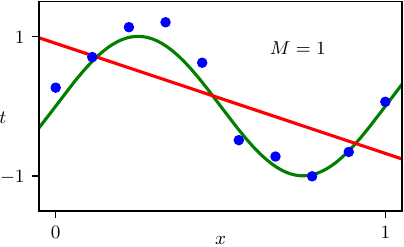
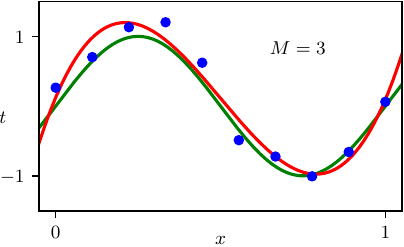
Bishop Fig 1.6 — the red line is the model we fit

The model: a polynomial of degree \(M\)

\[ y(x, \vw) = w_0 + w_1 x + w_2 x^2 + \dots + w_M x^M = \sum_{j=0}^{M} w_j x^j \]

Note: this function is nonlinear in \(x\) but linear in the parameters \(\vw\) — a property that makes it easy to solve (we return to this in the next session on regression).

We measure error with the sum-of-squares error:

\[ E(\vw) = \frac{1}{2}\sum_{n=1}^{N}\big\{ y(x_n,\vw) - t_n \big\}^2 \]

Best \(\vw\) = least squares

Minimize \(E(\vw)\) by setting the derivative to zero:

\[ \frac{\partial E}{\partial w_j} = \sum_{n=1}^{N}\big\{ y(x_n,\vw) - t_n \big\}\, x_n^{\,j} = 0 \]

Because \(E\) is quadratic in \(\vw\), the derivative is linear → a system of linear equations with a single closed-form solution.

This is a special case we can solve directly — most deep models cannot, so they rely on gradient descent (sessions 8–9).

Model complexity: which \(M\)?

\(M=9\) passes through every point exactly (\(E=0\)) but oscillates wildly — this is overfitting.

🔬 Demo: overfitting in code

import numpy as np, matplotlib.pyplot as plt
rng = np.random.default_rng(2)
x  = np.linspace(0, 1, 10)
t  = np.sin(2*np.pi*x) + 0.3*rng.standard_normal(10)   # 10 noisy points
xs = np.linspace(0, 1, 400)
plt.figure(figsize=(7.5, 2.6))
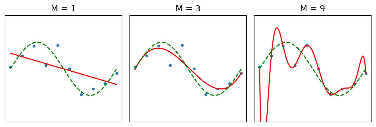
for i, M in enumerate([1, 3, 9]):
    if M == len(x) - 1:                                 # degree 9 with 10 points = exact interpolation
        w = np.linalg.solve(np.vander(x, M + 1), t); y = np.vander(xs, M + 1) @ w
    else:
        w = np.polyfit(x, t, M);                        y = np.polyval(w, xs)
    plt.subplot(1, 3, i + 1)
    plt.plot(x, t, "o", ms=3); plt.plot(xs, y, "r"); plt.plot(xs, np.sin(2*np.pi*xs), "g--")
    plt.title(f"M = {M}"); plt.ylim(-2, 2); plt.xticks([]); plt.yticks([])
plt.tight_layout(); plt.show()

Three lines of polyfit reproduce Bishop’s figure: M=1 underfits, M=3 is just right, M=9 overfits.

Measure on unseen data

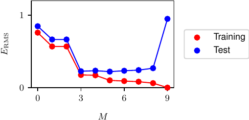
Training error keeps dropping as \(M\) grows
Test error drops then shoots back up at \(M=9\)
This gap = the generalization gap

The real goal is not to fit the training data, but to predict new data well.

🔬 Demo: train vs test error

import numpy as np, matplotlib.pyplot as plt
rng = np.random.default_rng(1)
def make(n): x = np.sort(rng.random(n)); return x, np.sin(2*np.pi*x) + 0.1*rng.standard_normal(n)
xtr, ttr = make(10)        # small training set
xte, tte = make(200)       # large unseen test set
rms = lambda w, x, t: np.sqrt(np.mean((np.polyval(w, x) - t)**2))
Ms  = range(0, 10)
tr  = [rms(np.polyfit(xtr, ttr, M), xtr, ttr) for M in Ms]
te  = [rms(np.polyfit(xtr, ttr, M), xte, tte) for M in Ms]
plt.figure(figsize=(5, 2.6))
plt.plot(list(Ms), tr, "o-", label="train"); plt.plot(list(Ms), te, "o-", label="test")
plt.xlabel("M"); plt.ylabel("RMS error"); plt.legend(); plt.tight_layout(); plt.show()

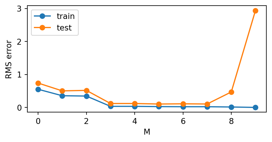
The test curve is U-shaped — minimum at moderate \(M\), blow-up at \(M=9\). We just measured the generalization gap.

More data helps

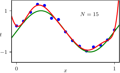
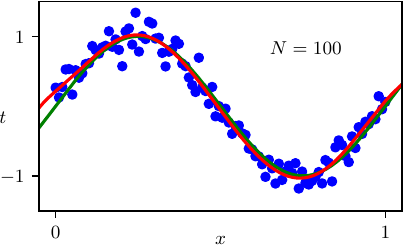
Same \(M=9\) model, but with more data (\(N\)) the overfitting fades — the right model complexity depends on how much data you have.

Controlling complexity with regularization

Add a penalty on large weights:

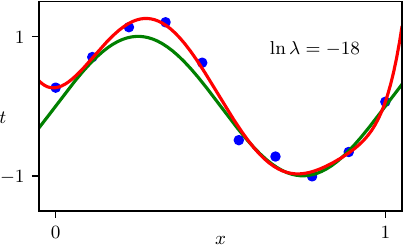
\[ \widetilde{E}(\vw) = \frac{1}{2}\sum_{n=1}^{N}\big\{ y(x_n,\vw) - t_n \big\}^2 + \frac{\lambda}{2}\,\norm{\vw}^2 \]

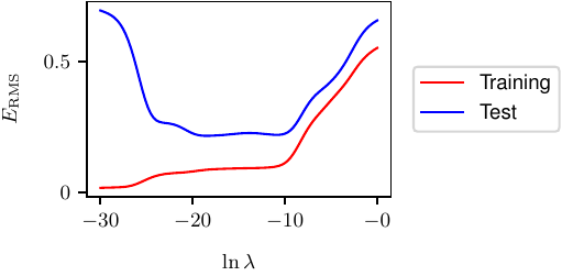
\(\lambda\) controls the trade-off: too small → overfit, too large → underfit. The sweet spot is in the middle (lowest test error).

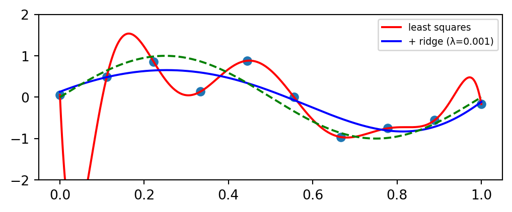
🔬 Demo: fit & regularize

import numpy as np, matplotlib.pyplot as plt
rng = np.random.default_rng(2)
x = np.linspace(0, 1, 10)
t = np.sin(2*np.pi*x) + 0.3*rng.standard_normal(10)

M   = 9            # ← try 3, 5, 9
lam = 1e-3         # ← try 0, 1e-5, 1e-3, 1.0

X = np.vander(x, M + 1)                                       # design matrix
w     = (np.linalg.solve(X, t) if M + 1 == len(x)            # plain least squares (overfits at M=9)
         else np.linalg.lstsq(X, t, rcond=None)[0])
w_reg = np.linalg.solve(X.T @ X + lam*np.eye(M + 1), X.T @ t) # + ridge penalty λ‖w‖²

xs = np.linspace(0, 1, 400); Xs = np.vander(xs, M + 1)
plt.figure(figsize=(5.4, 2.3))
plt.plot(x, t, "o"); plt.plot(xs, Xs@w, "r", label="least squares")
plt.plot(xs, Xs@w_reg, "b", label=f"+ ridge (λ={lam})"); plt.plot(xs, np.sin(2*np.pi*xs), "g--")
plt.ylim(-2, 2); plt.legend(fontsize=7); plt.tight_layout(); plt.show()

Part 5 · So Why Does “Depth” Work?

From one neuron to deep networks

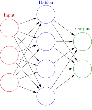
A neuron: a weighted sum of inputs, then a nonlinearity \(h\):

\[ z = h\!\Big(\underbrace{\textstyle\sum_{i=1}^{D} w_i x_i + b}_{\text{weighted sum}}\Big) = h(\vw^{\mathsf T}\vx + b) \]

\(w_i\) = weights, \(b\) = bias, \(h\) = activation (e.g. ReLU)
Stack neurons in layers → a neural network
“Deep” = many layers, each transforming the previous one’s features

Today’s polynomial had one layer of weights — depth is the next step.

Source: Wikimedia Commons — Colored neural network by Glosser.ca, CC BY-SA 3.0

A question that follows us all term

Today’s polynomial handles only a simple 1-D function. The real world (\(x\) = images, text) is far more complex.

Representation — a deep network learns features in layers, from simple to complex
Depth > Width — depth can represent some functions far more efficiently than width
Scale — more data + parameters + compute, in a principled way → predictably more capability

Summary

Deep learning = learning a function from data instead of writing rules by hand
The goal is generalization, not fitting the training data exactly → beware overfitting
Tools to control complexity: amount of data and regularization

Something to think about: the overfit \(M=9\) model has very large weights \(w_j\). Argue intuitively why the penalty term \(\tfrac{\lambda}{2}\norm{\vw}^2\) reduces overfitting — we will prove this formally in the regularization lecture.

📌 Read before next class

Required reading — there will be a reading quiz next session:

LeCun, Bengio & Hinton (2015), “Deep Learning”, Nature 521, 436–444

👉 nature.com/articles/nature14539

Next session: Mathematical Foundations — the probability toolkit we use all term (skim textbook Ch. 2).

As you read, be ready to answer:

What do the authors mean by representation learning, and why does it matter?
Why did deep learning succeed where hand-engineered features struggled?
What role do depth and large datasets play?