\( \newcommand{\vw}{\mathbf{w}} \newcommand{\vx}{\mathbf{x}} \newcommand{\vt}{\mathbf{t}} \newcommand{\vy}{\mathbf{y}} \newcommand{\vz}{\mathbf{z}} \newcommand{\vq}{\mathbf{q}} \newcommand{\vk}{\mathbf{k}} \newcommand{\vv}{\mathbf{v}} \newcommand{\vc}{\mathbf{c}} \newcommand{\vp}{\mathbf{p}} \newcommand{\vh}{\mathbf{h}} \newcommand{\vmu}{\boldsymbol{\mu}} \newcommand{\vsigma}{\boldsymbol{\sigma}} \newcommand{\vepsilon}{\boldsymbol{\epsilon}} \newcommand{\R}{\mathbb{R}} \newcommand{\E}{\mathbb{E}} \newcommand{\norm}[1]{\lVert #1 \rVert} \newcommand{\given}{\,\vert\,} \)

Lecture 9 — Convolutional Networks

Deep Learning · Session 9

Kasemsit Teeyapan

Department of Computer Engineering, Chiang Mai University

Today

  1. Why a fully-connected net is the wrong tool for images
  2. Convolution = local receptive fields + weight sharing (an inductive bias)
  3. Translation equivariance, padding, stride, channels
  4. Pooling and stacking → hierarchical features
  5. What CNNs learn, and the architectures that won: LeNet → AlexNet → VGG → ResNet

Reference: Bishop & Bishop (2024), Chapter 10Convolutional Networks

Recap → why a new architecture?

  • L5: the MLP — every unit connects to every input
  • L8: generalization comes from the right inductive bias
  • Images have structure an MLP throws away:
    • nearby pixels are related (locality)
    • a cat is a cat anywhere in the frame (translation)

A \(224\times224\times3\) image into a fully-connected layer of 1000 units:

\[224\cdot224\cdot3 \cdot 1000 \approx 1.5\times10^{8} \text{ weights}\]

…in one layer. And it learns “cat at top-left” separately from “cat at bottom-right.”

The fix: convolution

A small filter (kernel) slides across the image. Each output = a weighted sum of a local patch — and the same weights are reused everywhere.

\[z_{i,j} = \sum_{u,v} w_{u,v}\, x_{\,i+u,\;j+v}\]

  • Local receptive field — each unit sees a small patch
  • Weight sharing — one filter, reused at every position

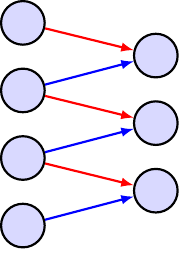
A convolution is a sparse, weight-shared layer: same colours = same weight.

Pillar: convolution = a fully-connected layer with two hard constraints — sparse connectivity + tied weights. Those constraints are the inductive bias.

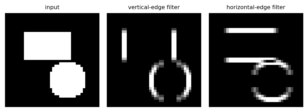
A filter is a feature detector

The weights are the feature. A hand-set edge filter:

\[K=\begin{bmatrix}-1&0&1\\-2&0&2\\-1&0&1\end{bmatrix}\]

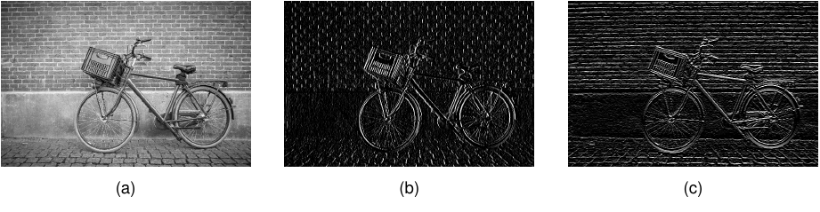
responds strongly where intensity changes left-to-right → vertical edges. Its transpose finds horizontal edges.

Source: Bishop & Bishop (2024), Fig 10.4 — (a) input, (b) horizontal-, (c) vertical-edge filter.

Demo: convolution from scratch

import numpy as np, matplotlib.pyplot as plt

img = np.zeros((40, 40))
img[8:20, 8:28] = 1.0                                   # a rectangle
yy, xx = np.mgrid[0:40, 0:40]
img[(yy - 28)**2 + (xx - 26)**2 < 64] = 1.0            # a disk

def conv2d(x, k):
    kh, kw = k.shape
    out = np.zeros((x.shape[0]-kh+1, x.shape[1]-kw+1))
    for i in range(out.shape[0]):
        for j in range(out.shape[1]):
            out[i, j] = np.sum(x[i:i+kh, j:j+kw] * k)
    return out

Kx = np.array([[-1,0,1],[-2,0,2],[-1,0,1]])            # vertical edges
gx, gy = conv2d(img, Kx), conv2d(img, Kx.T)            # Kx.T → horizontal

fig, ax = plt.subplots(1, 3, figsize=(6.2, 2.2))
for a, im, t in zip(ax, [img, np.abs(gx), np.abs(gy)],
                    ["input", "vertical-edge filter", "horizontal-edge filter"]):
    a.imshow(im, cmap="gray"); a.set_title(t, fontsize=8); a.axis("off")
plt.tight_layout(); plt.show()
Translation equivariance

Shift the input → the feature map shifts the same way:

\[\text{conv}(\text{shift}(x)) = \text{shift}(\text{conv}(x))\]

  • A filter that finds an edge finds it anywhere — for free
  • One filter is trained once, reused at every location
  • Add pooling (next) → approximate translation invariance

Equivariance (conv): output moves with the input.

Invariance (after pooling): output unchanged by small shifts.

Padding & stride

Padding — add a border of zeros so the output keeps the input size.

  • valid (none): output shrinks by \(K-1\)
  • same: pad so output size = input size

Stride — move the filter by \(s\) pixels each step.

  • \(s=1\): dense; \(s=2\): down-sample by ~2×

Output size for input \(W\), filter \(K\), padding \(P\), stride \(s\):

\[\left\lfloor \frac{W - K + 2P}{s} \right\rfloor + 1\]

VGG: \(3\times3\) filters, stride 1, same padding; down-sampling done by pooling.

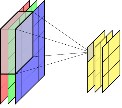
Channels: stacking filters

  • Input has channels (RGB = 3). A filter spans all input channels: a \(3\times3\) filter on RGB has \(3\cdot3\cdot3=27\) weights \((+1\) bias\()\).
  • Use many filters → many output feature maps (channels).
  • Each output channel = one learned feature detector.

Source: Bishop & Bishop (2024), Fig 10.7 — a multi-channel convolutional layer.

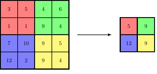
Pooling: down-sampling

Max-pooling takes the max over each small window.

  • shrinks resolution → fewer computations
  • gives local translation invariance (small shift, same max)
  • no learnable parameters

Source: Bishop & Bishop (2024), Fig 10.8 — \(2\times2\) max-pooling.

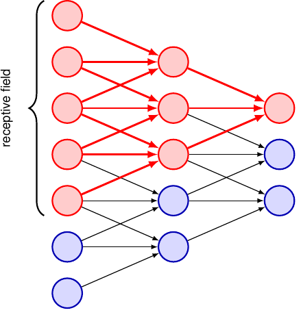
Stacking layers → hierarchy

Stack conv layers → a unit deep in the net has a large receptive field built from small filters.

  • layer 1 sees \(3\times3\)
  • layer 2 sees \(5\times5\) of the input
  • …depth grows the field cheaply

Source: Bishop & Bishop (2024), Fig 10.9 — receptive field grows with depth.

What do CNNs actually learn?

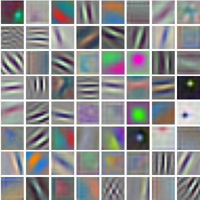
Fig 10.12 — learned first-layer filters: edges, colours, textures.

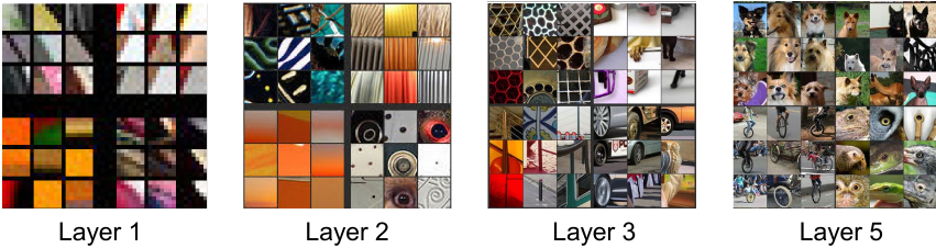
Fig 10.13 — patches that most activate units: edges → textures → parts → objects.

The representation-learning payoff (L5): nobody programmed “edge,” “eye,” or “dog.” The hierarchy emerged from data + the convolutional inductive bias.

Demo: why convolution wins on parameters

H, W, Cin, Cout = 224, 224, 3, 64

fc   = (H*W*Cin) * (H*W*Cout)        # fully-connected, same in/out spatial size
conv = (3*3*Cin + 1) * Cout          # one 3x3 conv layer, weights shared

print(f"Fully-connected layer : {fc:,} weights")
print(f"3x3 conv layer        : {conv:,} weights")
print(f"Ratio                 : {fc/conv:,.0f}x fewer")
Fully-connected layer : 483,385,147,392 weights
3x3 conv layer        : 1,792 weights
Ratio                 : 269,746,176x fewer

Same expressive job on a \(224\times224\) image — weight sharing turns \(10^{11}\) into \(10^{3}\).

Putting it together: a CNN

A typical classifier (e.g. VGG-16):

[conv → ReLU] × n → pool repeated, then flatten → fully-connected → softmax.

  • channels grow (64 → 128 → 256 → 512) as resolution shrinks via pooling
  • conv layers = feature extractor; FC head = classifier

LeNet (1998) — digits

AlexNet (2012) — won ImageNet; ReLU + dropout + GPUs

VGG (2014) — deep, all \(3\times3\)

ResNet (2015) — residuals → 100+ layers

The architecture race

ImageNet top-5 error:

  • pre-2012 (no deep CNN): ~26%
  • AlexNet (2012): 15.3%
  • deeper CNNs by ~2015: ~3.5%
  • human-level: ~5%

The 2012 jump wasn’t a new theory — it was the right inductive bias (convolution) + scale (ImageNet, GPUs) + regularization (ReLU, dropout, L8).

Summary

  1. Convolution = local receptive fields + weight sharing — a built-in inductive bias for images
  2. Translation equivariance (conv) → invariance (after pooling)
  3. Channels stack filters; pooling down-samples; depth grows receptive fields
  4. CNNs learn a feature hierarchy: edges → textures → parts → objects (L5)
  5. LeNet → AlexNet → VGG → ResNet: inductive bias + scale + regularization

Something to think about: convolution is equivariant to translation but not to rotation or scale. How would you build invariance to those? (Hint: data augmentation — L8 — or a different architecture.)

📌 Read before next class

Bishop & Bishop (2024), Chapter 12Transformers

From hard-wired image biases to learned attention: how to let the network decide what to relate to what.

References: LeCun et al. (1998) LeNet · Krizhevsky et al. AlexNet (2012) · Simonyan & Zisserman VGG (2014) · He et al. ResNet (2016) · Zeiler & Fergus Visualizing CNNs (2014). Figures from Bishop & Bishop (2024), Ch 10 — https://www.bishopbook.com/

⌂ Home