\( \newcommand{\vw}{\mathbf{w}} \newcommand{\vx}{\mathbf{x}} \newcommand{\vt}{\mathbf{t}} \newcommand{\vy}{\mathbf{y}} \newcommand{\vz}{\mathbf{z}} \newcommand{\vq}{\mathbf{q}} \newcommand{\vk}{\mathbf{k}} \newcommand{\vv}{\mathbf{v}} \newcommand{\vc}{\mathbf{c}} \newcommand{\vp}{\mathbf{p}} \newcommand{\vh}{\mathbf{h}} \newcommand{\vmu}{\boldsymbol{\mu}} \newcommand{\vsigma}{\boldsymbol{\sigma}} \newcommand{\vepsilon}{\boldsymbol{\epsilon}} \newcommand{\R}{\mathbb{R}} \newcommand{\E}{\mathbb{E}} \newcommand{\norm}[1]{\lVert #1 \rVert} \newcommand{\given}{\,\vert\,} \)

Lecture 6 — Gradient Descent

Deep Learning · Session 6

Kasemsit Teeyapan

Department of Computer Engineering, Chiang Mai University

Today

  1. The error surface \(E(\vw)\) and why we descend it
  2. Gradient descent and the all-important learning rate
  3. Batch · stochastic · mini-batch — and why noise helps
  4. Faster convergence: momentum, Adam, learning-rate schedules
  5. Why does Adam converge faster than SGD? — the question from Lecture 0

Reference: Bishop & Bishop (2024), Chapter 7Gradient Descent

Recap → why we need this

Lectures 2–3: linear models → \(\vw\) has a closed form (normal equations)

Lecture 5: a deep net’s \(E(\vw)\) is non-convex, no closed form

So we search for a minimum, step by step:

\[ \vw \leftarrow \vw - \eta\,\nabla E(\vw) \]

— follow the slope downhill.

Almost every deep network is trained by some flavor of gradient descent — understanding it is non-negotiable

Part 1 · The Error Surface

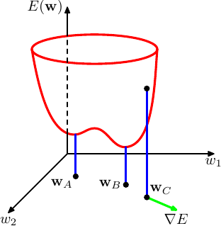
E(w) is a landscape over weight space

  • \(E(\vw)\) = a surface over all weights
  • \(\nabla E\) points uphill → step the opposite way
  • \(\nabla E = 0\) at minima, maxima, saddle points
  • deep nets: non-convex, many critical points

Near a minimum, \(E\) looks like a bowl (local quadratic) — the bowl’s shape decides how hard descent is.

Source: Bishop & Bishop (2024), Deep Learning, Fig 7.1

Conditioning: why the bowl shape matters

Toy bowl: \(E(x,y)=\tfrac12\big(x^2 + 100\,y^2\big)\).

  • steep in \(y\) (slope \(\times100\)), flat in \(x\)
  • to avoid diverging in \(y\), \(\eta\) must stay small → progress in \(x\) crawls
  • GD zig-zags down a long valley

In general: near a minimum \(E(\vw)\approx \tfrac12(\vw-\vw^\star)^\top H (\vw-\vw^\star)\), set by the Hessian \(H\).

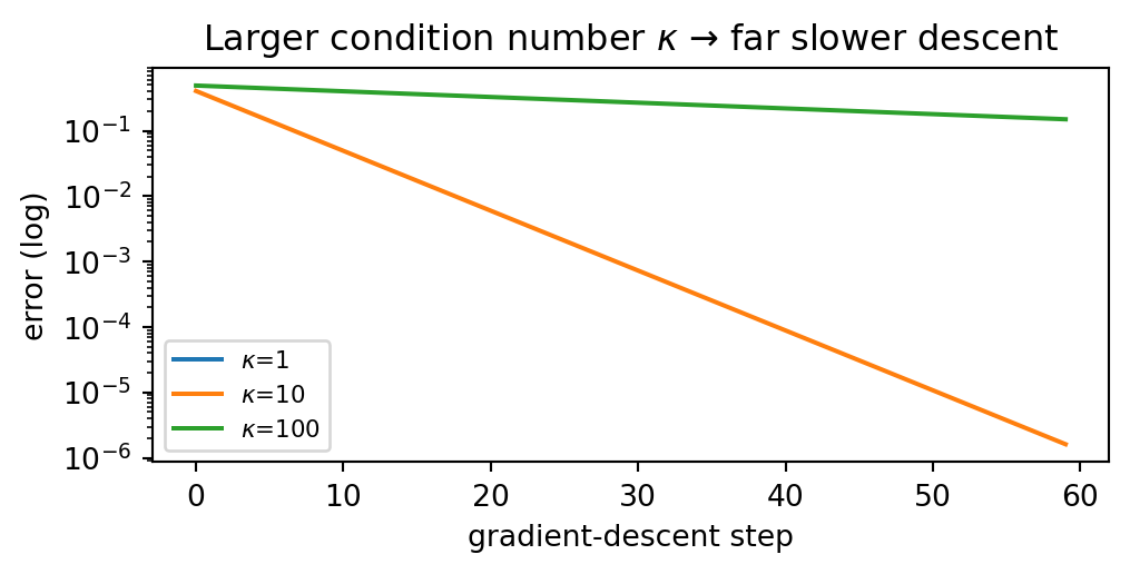
The condition number \(\kappa=\lambda_{\max}/\lambda_{\min}\) (here \(100/1=100\)) sets the speed: \[\text{error}\times\Big(\tfrac{\kappa-1}{\kappa+1}\Big)\text{ per step}\]

\(\eta\) is capped by the steep \(y\)-axis (push harder and \(y\) diverges). At that largest safe \(\eta\), how much does the flat \(x\)-direction shrink per step — 50%, 10%, or under 2%?

Pillar: GD is slow not because of how deep the valley is, but how elongated it is (\(\kappa\) large). This is exactly what momentum / Adam fix — they precondition away \(\kappa\).

🔬 Demo: convergence vs condition number

import numpy as np, matplotlib.pyplot as plt
plt.figure(figsize=(5.4,2.8))
for kappa in [1, 10, 100]:
    l = np.array([1.0, kappa]); eta = 1.0/l.max()       # eigenvalues; lr set by steepest
    w = np.array([1.0, 1.0]); errs = []
    for _ in range(60):
        w = w - eta*(l*w); errs.append(0.5*np.sum(l*w**2))
    plt.semilogy(errs, label=f"$\\kappa$={kappa}")
plt.xlabel("gradient-descent step"); plt.ylabel("error (log)")
plt.title("Larger condition number $\\kappa$ → far slower descent"); plt.legend(fontsize=8)
plt.tight_layout(); plt.show()

Conditioning by the numbers

\(E(x,y)=\tfrac12(x^2+100y^2)\), gradient \((x,\,100y)\), so \(\kappa=100\).

  1. Stability in \(y\) needs \(\eta<2/\lambda_{\max}=2/100=0.02\). Take \(\eta=0.018\).
  2. Steep \(y\): factor \(1-0.018\times100=-0.8\) → collapses fast.
  3. Flat \(x\): factor \(1-0.018\times1=0.982\) → shrinks only 1.8% per step.
  4. So \(x\) needs \(\approx38\) steps just to halve (\(0.982^{38}\approx0.5\)).

The steep axis sets \(\eta\); the flat axis pays for it — exactly the \(\kappa=100\) crawl in the demo. Under 2% — did your guess match?

Same bowl but \(\kappa=10\): \(E=\tfrac12(x^2+10y^2)\). What is the largest safe \(\eta\)? Using \(\eta=0.18\), give the \(x\)- and \(y\)-factors and how many steps \(x\) needs to halve.

Saddle points, not bad minima

At a critical point (\(\nabla E=0\)), it’s a minimum only if all \(D\) Hessian eigenvalues are positive.

In high dimensions that’s like \(D\) coin-flips all landing heads → exponentially rare.

So most critical points are saddle points, not local minima — and the few minima are usually near-global. The real enemy of deep-net optimization is saddles & plateaus, not getting trapped in a bad valley.

In \(D=10\) dimensions, if each Hessian eigenvalue is positive or negative like a coin flip, what’s the chance a random critical point is a true minimum?

All \(10\) must be positive: \((1/2)^{10}=1/1024\approx\mathbf{0.1\%}\). At \(D=10^6\) weights it is \(2^{-10^6}\) — effectively zero. Saddles everywhere; genuine minima almost never.

Dauphin et al. (2014); Choromanska et al. (2015) — the prevalence of saddle points in high-dimensional losses

Part 2 · Gradient Descent & the Learning Rate

The learning rate makes or breaks it

\[ \vw \leftarrow \vw - \eta\,\nabla E(\vw) \qquad (\eta = \text{learning rate}) \]

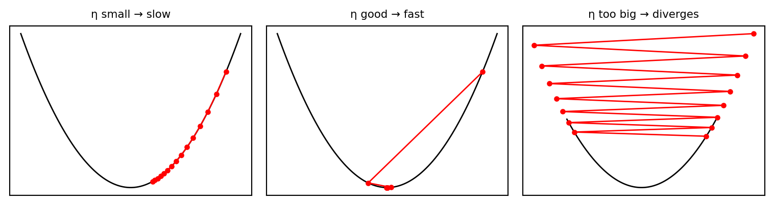
GD on the bowl \(E(w)=w^2\) from \(w=1\) gives \(w\leftarrow(1-2\eta)w\). As \(\eta\) grows from \(0\), at what value do the steps stop shrinking and start to blow up?

import numpy as np, matplotlib.pyplot as plt
f = lambda w: w**2; g = lambda w: 2*w; xs = np.linspace(-3, 3, 100)
fig, ax = plt.subplots(1, 3, figsize=(8, 2.2))
for a, (lr, ttl) in zip(ax, [(0.05, "η small → slow"), (0.6, "η good → fast"),
                             (1.02, "η too big → diverges")]):
    w = 2.6; ws = [w]
    for _ in range(14): w = w - lr*g(w); ws.append(w)
    a.plot(xs, f(xs), "k", lw=1); a.plot(ws, [f(v) for v in ws], "o-", color="r", ms=3, lw=1)
    a.set_title(ttl, fontsize=8); a.set_xticks([]); a.set_yticks([])
plt.tight_layout(); plt.show()
Too small → crawls; too large → overshoots and diverges. The single most important hyperparameter.

Learning rate by the numbers

\(E(w)=w^2\), so \(\nabla E=2w\) and \(w\leftarrow w-\eta\,2w=(1-2\eta)w\). Take \(\eta=0.1\), \(w_0=1\):

step \(w\) \(E=w^2\)
0 1 1
1 0.8 0.64
2 0.64 0.41
3 0.512 0.26

Each step scales \(w\) by \(|1-2\eta|=0.8<1\) → converges. It blows up once \(|1-2\eta|\ge1\), i.e. \(\eta\ge1=2/a\) (here \(a=2\)) — that’s the threshold you predicted.

Same bowl, \(w_0=1\). (a) With \(\eta=0.4\), write \(w_1,w_2,w_3\) — converge or diverge? (b) And with \(\eta=1.2\)?

Part 3 · Batch, Stochastic, Mini-batch

How many examples per step?

\(E(\vw)=\sum_{n=1}^N E_n(\vw)\) — computing the full gradient every step is expensive.

  • Batch: all \(N\) → accurate but slow
  • Stochastic (SGD): one \(E_n\) → noisy but cheap
  • Mini-batch: a small group (e.g. 32–256) → the practical standard

The noise in SGD is a feature:

  • escapes saddle points & sharp minima
  • often generalizes better
  • enables training on huge datasets

A mini-batch of \(100\) examples vs a single one: the gradient estimate’s noise (standard deviation) drops by what factor?

Mini-batch SGD — noisy, cheap steps — is how essentially all deep nets are trained

Part 4 · Faster Convergence

Momentum accelerates slow directions

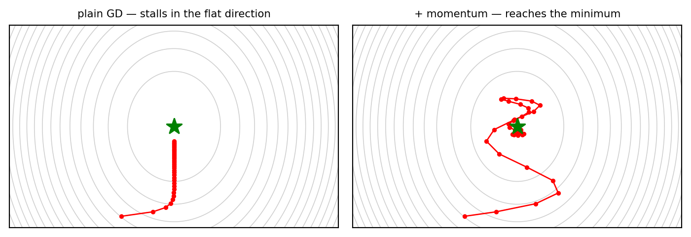
In a ravine, plain GD takes tiny steps along the shallow direction. Momentum builds up velocity there:

\[ \mathbf v \leftarrow \mu\,\mathbf v - \eta\,\nabla E, \qquad \vw \leftarrow \vw + \mathbf v \]

Along a shallow valley floor the gradient is a small constant. Plain GD inches forward by \(\eta g\) each step. With \(\mu=0.9\), how big does each step eventually get — the same, \(2\times\), or \(10\times\)?

Same \(\eta\): plain GD barely moves along the flat axis, while momentum builds speed and reaches the minimum.

cf. Bishop & Bishop (2024), Deep Learning, Figs 7.3 & 7.6

Momentum by the numbers

Constant gradient \(g=1\) along a flat direction, \(\eta=0.1\), \(\mu=0.9\), start \(v=0\), using \(v\leftarrow\mu v-\eta g\):

step \(v\)
1 \(-0.1\)
2 \(-0.19\)
3 \(-0.271\)
4 \(-0.344\)

The velocity saturates at \(v_\infty=-\dfrac{\eta g}{1-\mu}=-\dfrac{0.1}{0.1}=-1.0\) — a \(10\times\) bigger step than plain GD’s \(-0.1\). That is the ravine speed-up in the plot.

Momentum multiplies the speed in any steady direction by \(\tfrac{1}{1-\mu}\): \(\mu=0.9\Rightarrow10\times\), \(\mu=0.99\Rightarrow100\times\).

Repeat with \(\mu=0.8\) (same \(\eta,g\)). What is the terminal velocity \(v_\infty\), and how many times the plain step is it?

Adam: a learning rate per parameter

RMSProp/Adam scale each coordinate by its own recent gradient size:

\[ \mathbf m \leftarrow \beta_1\mathbf m + (1-\beta_1)\,\mathbf g, \qquad \mathbf v \leftarrow \beta_2\mathbf v + (1-\beta_2)\,\mathbf g^2 \] \[ \vw \leftarrow \vw - \eta\,\frac{\hat{\mathbf m}}{\sqrt{\hat{\mathbf v}}+\epsilon} \qquad (\hat{\mathbf m},\hat{\mathbf v}\text{ = bias-corrected}) \]

  • \(\mathbf m\) = momentum (1st moment) · \(\mathbf v\) = gradient size (2nd moment)
  • big-gradient directions get smaller steps; small-gradient directions get bigger steps

On the first step (\(m,v\) start at \(0\), then bias-corrected), weight A has gradient \(g=0.5\) and weight B has \(g=50\). Which one takes the bigger step?

Bishop §7.3.3 · Kingma & Ba, Adam (2015)

Adam by the numbers

First step, \(\beta_1=0.9,\ \beta_2=0.999,\ \eta=0.001\), gradient \(g=0.5\):

  1. \(m=(1-\beta_1)g=0.1\times0.5=0.05\), \(\quad v=(1-\beta_2)g^2=0.001\times0.25=0.00025\)
  2. bias-correct: \(\hat m=m/(1-\beta_1)=0.5\), \(\quad\hat v=v/(1-\beta_2)=0.25\)
  3. step \(=\eta\,\hat m/\sqrt{\hat v}=0.001\times0.5/0.5=\mathbf{0.001}=\eta\)

Redo with \(g=50\): \(\hat m=50,\ \hat v=2500,\ \sqrt{\hat v}=50\) → step \(=0.001\times50/50=\mathbf{0.001}\). Same step — A and B move together.

On the first step Adam moves \(\approx\eta\cdot\operatorname{sign}(g)\) in every coordinate — the per-parameter rate erases gradient scale (this is what fixes conditioning).

Two parameters on the first Adam step: \(g_1=0.1\) and \(g_2=10\). Compute each step size. Which weight moves further?

Why does Adam converge faster than SGD?

The mechanism

  • it rescales each axis by its gradient size → an ill-conditioned bowl looks round → no zig-zag
  • robust to very different gradient scales (sparse / NLP features)
  • works well with little tuning of \(\eta\)

The honest caveat

  • SGD + momentum often generalizes better (esp. vision) → still used for ResNets
  • Adam dominates Transformers / LLMs
  • “faster” = fewer steps to low training loss, not always better test error

Adam fixes conditioning automatically — but the right optimizer is empirical, not universal (the judgement this course builds)

Learning-rate schedules

A fixed \(\eta\) is rarely best — change it during training:

  • decay (step / cosine): large steps early to explore, small steps late to settle
  • warmup: start tiny for a few hundred steps (stabilizes Adam / Transformers)

Schedules are why “the same model” trains far better with a good \(\eta(t)\) — a key practical lever.

Bishop §7.3.2 · normalization (batch / layer norm) also eases optimization — we cover it with regularization

Summary

  1. Train by descending the error surface: \(\vw \leftarrow \vw - \eta\nabla E\) — the learning rate is critical
  2. Mini-batch SGD: noisy, cheap steps; the noise even helps generalization
  3. Momentum cancels zig-zag; Adam gives a per-parameter rate (fixes conditioning)
  4. The best optimizer & schedule are empirical — Adam for Transformers, SGD+momentum often for vision

Something to think about: on the bowl \(E(w)=\tfrac12 a w^2\), GD is \(w\leftarrow(1-\eta a)w\). For what range of \(\eta\) does it converge? What happens at \(\eta=2/a\)? (This is why curvature sets the safe step.)

📌 Read before next class

Bishop & Bishop (2024), Chapter 8Backpropagation

Gradient descent needs \(\nabla E\). For a deep net with millions of weights, how do we compute it efficiently? The chain rule, run backwards.

Figures from Bishop & Bishop, Deep Learning: Foundations and Concepts (2024), Chapter 7 — https://www.bishopbook.com/

⌂ Home