\( \newcommand{\vw}{\mathbf{w}} \newcommand{\vx}{\mathbf{x}} \newcommand{\vt}{\mathbf{t}} \newcommand{\vy}{\mathbf{y}} \newcommand{\vz}{\mathbf{z}} \newcommand{\vq}{\mathbf{q}} \newcommand{\vk}{\mathbf{k}} \newcommand{\vv}{\mathbf{v}} \newcommand{\vc}{\mathbf{c}} \newcommand{\vp}{\mathbf{p}} \newcommand{\vh}{\mathbf{h}} \newcommand{\vmu}{\boldsymbol{\mu}} \newcommand{\vsigma}{\boldsymbol{\sigma}} \newcommand{\vepsilon}{\boldsymbol{\epsilon}} \newcommand{\R}{\mathbb{R}} \newcommand{\E}{\mathbb{E}} \newcommand{\norm}[1]{\lVert #1 \rVert} \newcommand{\given}{\,\vert\,} \)

Lecture 12 — Generative Models

Deep Learning · Session 12

Kasemsit Teeyapan

Department of Computer Engineering, Chiang Mai University

Today

  1. From discriminative \(p(t\mid\vx)\) to generative \(p(\vx)\) — learn the data itself
  2. VAEs — a probabilistic autoencoder; ELBO + the reparameterization trick
  3. GANs — a generator vs a discriminator (adversarial training)
  4. Diffusion — add noise, then learn to remove it
  5. How the three families trade off, and what powers modern image generation

Reference: Bishop & Bishop (2024), Ch 17 (GANs), §19.2 (VAEs), Ch 20 (Diffusion)

Recap → why generate?

  • so far: discriminative\(p(t\mid\vx)\), a boundary
  • now: generative\(p(\vx)\), the whole distribution

Learning \(p(\vx)\) lets us:

  • sample new data (images, audio, text)
  • spot outliers (low \(p(\vx)\)L15)
  • learn structure without labels (L11)

\(\vx\) is huge (a \(256^2\) image lives in $$200k dimensions) and \(p(\vx)\) is wildly complex. We can’t write it down — we must learn to sample from it.

Three families

idea sampling
VAE latent + likelihood (ELBO) 1 pass
GAN adversarial game 1 pass
Diffusion iterative denoising many steps

All three learn a map from simple noise \(\vz\sim\mathcal N(0,I)\) to complex data \(\vx\).

They differ in how they train that map.

VAE: a probabilistic autoencoder

Take the autoencoder (L11) and make the latent probabilistic:

  • encoder outputs a distribution \(q(\vz\mid\vx)=\mathcal N(\vmu,\,\vsigma^2)\)
  • prior \(p(\vz)=\mathcal N(0,I)\) — so we can sample \(\vz\) and decode
  • decoder \(p(\vx\mid\vz)\) reconstructs

Maximize the evidence lower bound (ELBO):

\[\mathcal L = \underbrace{\E_{q}\!\left[\ln p(\vx\mid\vz)\right]}_{\text{reconstruction}} - \underbrace{\mathrm{KL}\!\left(q(\vz\mid\vx)\,\Vert\,p(\vz)\right)}_{\text{stay close to prior}}\]

Where the ELBO comes from

We want \(\ln p(\vx)\) but the integral \(\int p(\vx\given\vz)p(\vz)\,d\vz\) is intractable. Introduce \(q(\vz\given\vx)\) and apply Jensen’s inequality:

\[\ln p(\vx)=\ln\!\int q(\vz\given\vx)\frac{p(\vx,\vz)}{q(\vz\given\vx)}\,d\vz\] \[\ge \E_{q}\!\Big[\ln\frac{p(\vx,\vz)}{q(\vz\given\vx)}\Big]=\mathcal L\;(\text{ELBO})\]

The gap is exactly a KL: \[\ln p(\vx)-\mathcal L=\mathrm{KL}\big(q(\vz\given\vx)\,\Vert\,p(\vz\given\vx)\big)\ge 0\]

Pillar: maximizing the ELBO does two jobs at once — it pushes up \(\ln p(\vx)\) (fit the data) and drives \(q(\vz\given\vx)\) toward the true posterior \(p(\vz\given\vx)\). Expanding \(\mathcal L\) gives the reconstruction \(-\) KL form from the last slide.

VAE: the reparameterization trick

Problem: we must backprop (L7) through a sampling step \(\vz\sim q(\vz\mid\vx)\) — but sampling isn’t differentiable.

Trick: move the randomness outside:

\[\vz = \vmu + \vsigma \odot \vepsilon, \qquad \vepsilon\sim\mathcal N(0,I)\]

Pillar: now \(\vmu,\vsigma\) are deterministic outputs and gradients flow through them; the noise \(\vepsilon\) is just an input. This one trick makes VAEs trainable.

GAN: an adversarial game

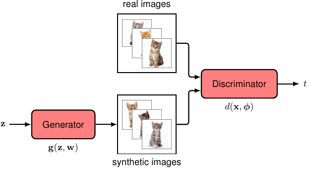
Two networks compete:

  • generator \(g(\vz)\) turns noise into fake data
  • discriminator \(d(\vx)\) judges real vs fake

\[\min_g \max_d\; \E_{\vx}[\ln d(\vx)] + \E_{\vz}[\ln(1 - d(g(\vz)))]\]

At equilibrium, fakes are indistinguishable from real — no explicit \(p(\vx)\) needed.

Source: Bishop & Bishop (2024), Fig 17.1 — generator vs discriminator.

GAN: sharp but tricky

  • + very sharp samples, fast 1-pass generation
  • unstable training (two moving objectives)
  • mode collapse — generator outputs only a few “safe” samples, ignoring diversity
  • no likelihood → hard to evaluate

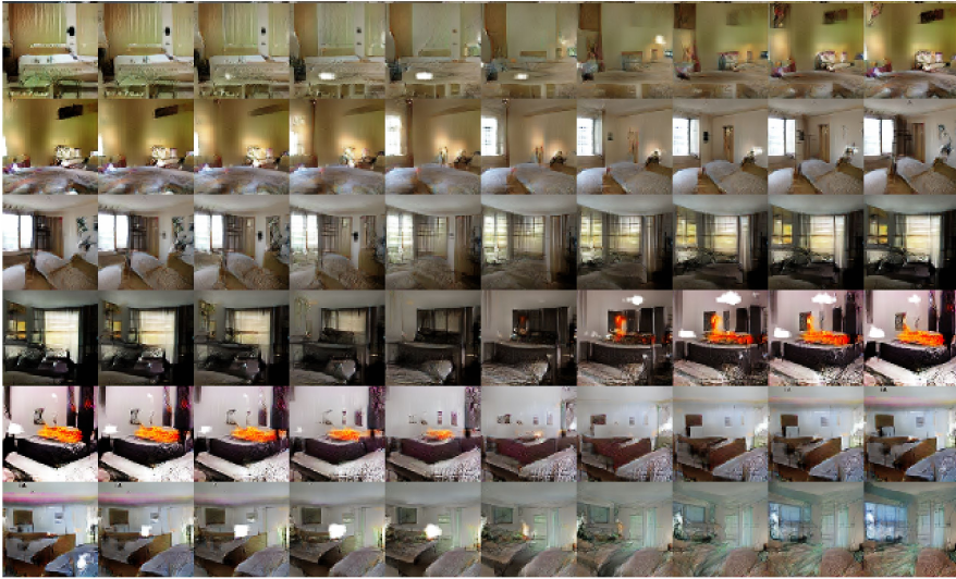
Source: Bishop & Bishop (2024), Fig 17.9 — DCGAN samples (bedroom images).

Diffusion: destroy, then restore

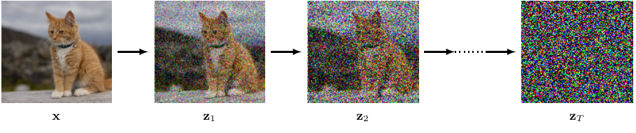
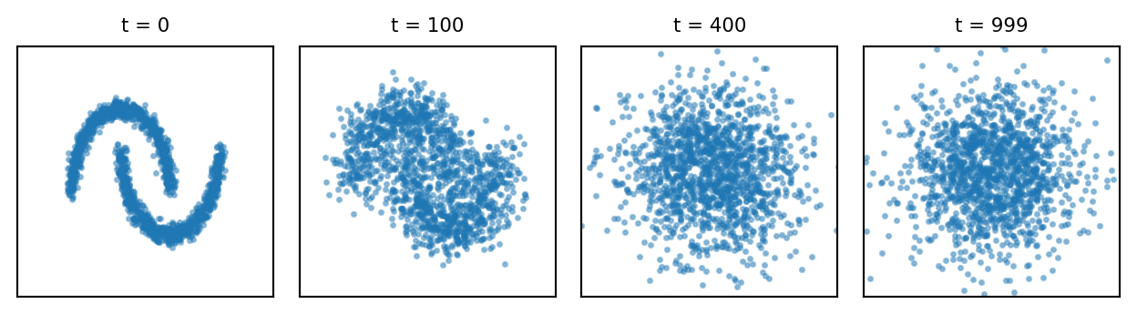
Forward (fixed): gradually add Gaussian noise over \(T\) steps until data → pure noise.

\[\vx_t = \sqrt{\bar\alpha_t}\,\vx_0 + \sqrt{1-\bar\alpha_t}\,\vepsilon\]

Reverse (learned): a network undoes one step at a time — trained simply to predict the noise:

\[E(w)=\norm{\vepsilon - \vepsilon_w(\vx_t, t)}^2\]

Source: Bishop & Bishop (2024), Fig 20.1 — forward process: \(\vx_0 \to \vz_T\) (noise).

Demo: the forward diffusion process

import numpy as np, matplotlib.pyplot as plt
from sklearn.datasets import make_moons

X, _ = make_moons(n_samples=1500, noise=0.06, random_state=0)
X = (X - X.mean(0)) / X.std(0)
betas = np.linspace(1e-4, 0.02, 1000); abar = np.cumprod(1 - betas)
rng = np.random.default_rng(0)

steps = [0, 100, 400, 999]
fig, ax = plt.subplots(1, 4, figsize=(6.6, 1.9))
for a_, t in zip(ax, steps):
    xt = np.sqrt(abar[t]) * X + np.sqrt(1 - abar[t]) * rng.normal(size=X.shape)
    a_.scatter(xt[:, 0], xt[:, 1], s=3, alpha=0.4)
    a_.set_title(f"t = {t}", fontsize=8); a_.set_xticks([]); a_.set_yticks([])
    a_.set_xlim(-3, 3); a_.set_ylim(-3, 3)
plt.tight_layout(); plt.show()
Diffusion: generation & guidance

Generate: start from noise \(\vz_T\sim\mathcal N(0,I)\), apply the learned denoiser \(T\) times → a fresh sample.

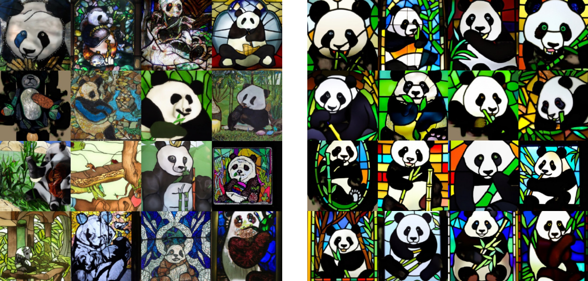
Guidance: condition on a prompt \(\vc\) (text). Classifier-free guidance dials how strongly to follow \(\vc\).

  • the denoiser is usually a U-Net (L9) or transformer (L10)

Source: Bishop & Bishop (2024), Fig 20.7 — classifier-free guidance: weak (left) → strong (right).

Pillar: diffusion = stable training + best diversity. It now powers most text-to-image and video models.

Choosing a family

sharpness diversity training speed
VAE blurry good stable fast
GAN sharp poor (collapse) unstable fast
Diffusion sharp best stable slow

No free lunch (L4 again): VAEs give likelihood but blur; GANs are sharp but fragile; diffusion wins quality at the cost of many sampling steps.

Summary

  1. Generative models learn \(p(\vx)\) — map simple noise \(\to\) complex data
  2. VAE = probabilistic autoencoder; ELBO + reparameterization trick make it trainable
  3. GAN = generator vs discriminator; sharp but unstable, mode collapse
  4. Diffusion = add noise, learn to predict & remove it; stable, diverse, slow
  5. Modern image/video gen = diffusion + U-Net/transformer + guidance + scale (L13)

Something to think about: VAE samples are often blurry. Why does maximizing the Gaussian reconstruction likelihood (an \(\ell_2\) term) encourage averaging over plausible images? (Hint: the mean minimizes expected squared error.)

📌 Read before next class

Scaling & Modern AI Systems

Scaling laws, compute-optimal training, and the emergence of capabilities in large language models.

Reading: Kaplan et al., Scaling Laws for Neural Language Models (2020); Hoffmann et al., Training Compute-Optimal LLMs (Chinchilla) (2022). References: Goodfellow et al., GAN (2014); Kingma & Welling, VAE (2014); Ho et al., DDPM (2020). Figures from Bishop & Bishop (2024), Ch 17/19/20 — https://www.bishopbook.com/

⌂ Home