\( \newcommand{\vw}{\mathbf{w}} \newcommand{\vx}{\mathbf{x}} \newcommand{\vt}{\mathbf{t}} \newcommand{\vy}{\mathbf{y}} \newcommand{\vz}{\mathbf{z}} \newcommand{\vq}{\mathbf{q}} \newcommand{\vk}{\mathbf{k}} \newcommand{\vv}{\mathbf{v}} \newcommand{\vc}{\mathbf{c}} \newcommand{\vp}{\mathbf{p}} \newcommand{\vh}{\mathbf{h}} \newcommand{\vmu}{\boldsymbol{\mu}} \newcommand{\vsigma}{\boldsymbol{\sigma}} \newcommand{\vepsilon}{\boldsymbol{\epsilon}} \newcommand{\R}{\mathbb{R}} \newcommand{\E}{\mathbb{E}} \newcommand{\norm}[1]{\lVert #1 \rVert} \newcommand{\given}{\,\vert\,} \)

Lecture 16 — Distribution Shift & OOD Generalization

Deep Learning · Session 16

Kasemsit Teeyapan

Department of Computer Engineering, Chiang Mai University

Today

  1. The assumption behind everything: train ≈ test (IID, from L4) — and how it breaks
  2. Types of distribution shift: covariate, label, concept
  3. Shortcut learning — models exploit spurious correlations
  4. OOD detection: the max-softmax baseline and why it fails
  5. The course comes full circle: from IID generalization (L4) to OOD generalization

Reading: Hendrycks & Gimpel (2017); Geirhos et al. (2020). This is paper-based — Bishop has no OOD chapter.

Recap → the hidden assumption

L4 built everything on i.i.d.: training and test data drawn from the same distribution \(p(\vx, y)\).

ERM minimizes empirical risk, trusting it approximates true risk — only if the distribution doesn’t change.

The real world is not i.i.d.: cameras change, hospitals differ, language drifts, users adapt. A model perfect on the test set can fail badly in deployment.

Types of distribution shift

  • Covariate shift\(p(\vx)\) changes, \(p(y\mid\vx)\) same
    • new camera, new lighting, new hospital
  • Label shift\(p(y)\) changes
    • disease prevalence rises in a new season
  • Concept drift\(p(y\mid\vx)\) changes
    • what counts as “spam” evolves

Each breaks a different part of the i.i.d. assumption — and each needs a different fix. Naming the shift is the first step.

Shortcut learning

Models take the easiest predictive cue — even if it’s spurious (Geirhos et al., 2020):

  • “cow” detector that really detects grass
  • pneumonia model reading the hospital’s scanner tag, not the lungs
  • ImageNet CNNs biased to texture, not shape

A shortcut gives great i.i.d. test accuracy (L4) but collapses under shift — the cue vanishes or flips. High accuracy hid a model that learned the wrong thing.

Detecting OOD inputs

Before trusting a prediction, ask: is this input even from the training distribution?

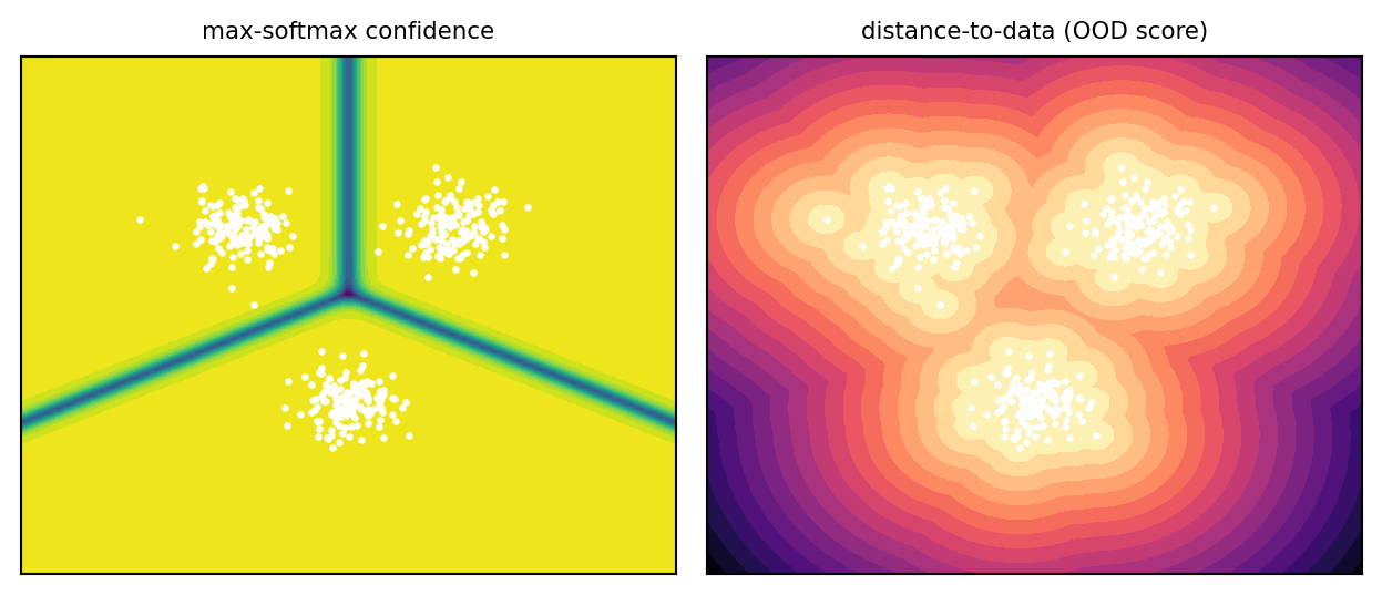
Max-softmax baseline (Hendrycks & Gimpel, 2017): flag inputs whose maximum softmax confidence is low.

  • simple, no retraining
  • but (L15): nets are overconfident — they stay confident far from any data

OOD detection = a binary task layered on top of the classifier: in-distribution vs out. Confidence is a starting point, not the answer.

Demo: where confidence fails

import numpy as np, matplotlib.pyplot as plt
from scipy.spatial import cKDTree
rng = np.random.default_rng(0)
sm = lambda z: np.exp(z-z.max(-1,keepdims=True))/np.exp(z-z.max(-1,keepdims=True)).sum(-1,keepdims=True)
centers = np.array([[3,3],[-3,3],[0,-3]], float)
Xtr = np.vstack([rng.normal(c, 0.7, (150,2)) for c in centers])
gx, gy = np.meshgrid(np.linspace(-9,9,120), np.linspace(-9,9,120)); G = np.c_[gx.ravel(), gy.ravel()]

conf = sm(-0.5*((G[:,None,:]-centers[None])**2).sum(-1)).max(1).reshape(gx.shape)   # max-softmax
dist = cKDTree(Xtr).query(G, k=1)[0].reshape(gx.shape)                               # distance to data

fig, ax = plt.subplots(1, 2, figsize=(6.6, 2.9))
for a, M, t, cm in [(ax[0], conf, "max-softmax confidence", "viridis"),
                    (ax[1], -dist, "distance-to-data (OOD score)", "magma")]:
    a.contourf(gx, gy, M, levels=20, cmap=cm); a.scatter(Xtr[:,0], Xtr[:,1], s=2, c="w")
    a.set_title(t, fontsize=8); a.set_xticks([]); a.set_yticks([])
plt.tight_layout(); plt.show()
Toward robustness

Detect the shift:

  • density / Mahalanobis / energy scores
  • outlier exposure (train on known OODs)

Survive the shift:

  • data augmentation (L8) — simulate the shifts you expect
  • domain generalization, invariant features
  • calibrated confidence (L15) → abstain

Pillar: there is no free lunch (L4) for arbitrary shift. Robustness comes from encoding what you expect to change — an inductive bias, again (L8/L9).

Full circle: it was all generalization

  • L4: generalization under i.i.d. — capacity, ERM, the bias–variance / VC story
  • L8L9: inductive bias to generalize better
  • L14: scaling — generalization as a power law
  • L16: generalization off-distribution — the open frontier

Every lecture was one question in disguise: when, and why, does what we learned from data transfer to data we haven’t seen?

Summary

  1. Everything assumed i.i.d. (L4); real deployment faces distribution shift
  2. Covariate / label / concept shift each break it differently
  3. Shortcut learning: high i.i.d. accuracy can hide the wrong solution
  4. Max-softmax OOD detection is a baseline; nets are overconfident off-distribution (L15)
  5. Robustness = detect + survive shift, by encoding expected invariances (L8) — no free lunch (L4)

The big question to carry forward: an LLM can write the code for any of these methods. Your job is to know which to use, why, and how to tell if it actually worked. That judgment is what this course was for.

📌 Looking ahead

You now have the theoretical spine of modern deep learning — from linear models to transformers, diffusion, scaling, and trustworthy deployment.

What’s next: read the papers deeply, reproduce a result, and question every confident number.

References: Hendrycks & Gimpel, OOD Baseline (2017); Geirhos et al., Shortcut Learning (2020); Lee et al., Mahalanobis OOD (2018); Liu et al., Energy-based OOD (2020).

⌂ Home