\( \newcommand{\vw}{\mathbf{w}} \newcommand{\vx}{\mathbf{x}} \newcommand{\vt}{\mathbf{t}} \newcommand{\vy}{\mathbf{y}} \newcommand{\vz}{\mathbf{z}} \newcommand{\vq}{\mathbf{q}} \newcommand{\vk}{\mathbf{k}} \newcommand{\vv}{\mathbf{v}} \newcommand{\vc}{\mathbf{c}} \newcommand{\vp}{\mathbf{p}} \newcommand{\vh}{\mathbf{h}} \newcommand{\vmu}{\boldsymbol{\mu}} \newcommand{\vsigma}{\boldsymbol{\sigma}} \newcommand{\vepsilon}{\boldsymbol{\epsilon}} \newcommand{\R}{\mathbb{R}} \newcommand{\E}{\mathbb{E}} \newcommand{\norm}[1]{\lVert #1 \rVert} \newcommand{\given}{\,\vert\,} \)

Lecture 4 — Statistical Learning & Generalization

Deep Learning · Session 4

Kasemsit Teeyapan

Department of Computer Engineering, Chiang Mai University

Today

  1. What we really minimize: risk (true vs empirical)
  2. Overfitting, model capacity, and the bias–variance trade-off
  3. How much can a model fit? VC dimension (intuition) & Occam’s razor
  4. Generalization bounds (conceptual) — and the modern puzzle of deep nets

References: Bishop & Bishop (2024) §4.3 (bias–variance); Shalev-Shwartz & Ben-David, Understanding Machine Learning (ERM, capacity, VC)

Part 1 · What We Really Minimize

True risk vs empirical risk

We want low error on the whole data distribution \(p(\vx,t)\) — the true (expected) risk:

\[ R(f) = \mathbb{E}_{(\vx,t)\sim p}\big[\,L(f(\vx), t)\,\big] \]

But we only have \(N\) samples, so we minimize the empirical risk (training loss):

\[ R_{\text{emp}}(f) = \frac{1}{N}\sum_{n=1}^{N} L\big(f(\vx_n), t_n\big) \qquad\text{(ERM)} \]

Here \(f\) is our model \(y(\vx,\vw)\) and \(L\) is the loss from Lectures 1–3 (squared error or cross-entropy). \(R_{\text{emp}}\) is just the average training error \(E(\vw)/N\) we have been minimizing.

The generalization gap \(= R(f) - R_{\text{emp}}(f)\) is what all of learning theory tries to bound

Why a gap appears

  • ERM drives training error down
  • But a flexible model can fit noise, not just signal
  • → low train error, high true risk = overfitting
  • Too rigid a model can’t fit the signal either
  • → high train and test error = underfitting

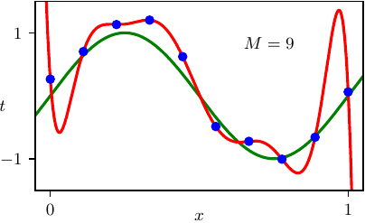
We saw this concretely in Lecture 0: the \(M=9\) polynomial passes through every point (\(R_{\text{emp}}\approx 0\)) yet swings wildly → high true risk. Today: why it happens, in general.

Source: Bishop & Bishop (2024), Deep Learning, Fig 1.6 (\(M=9\)) — the overfitting example from Lecture 0

Part 2 · Capacity & the Bias–Variance Trade-off

Model capacity

Capacity = how rich the hypothesis class \(\mathcal F\) — the set of all functions the model can represent — is (e.g. all degree-\(M\) polynomials; all linear classifiers).

  • Low capacity → high bias (misses the pattern)
  • High capacity → high variance (sensitive to the particular training sample)
  • The right capacity depends on how much data you have

Generalization is a balance between fitting the data and staying simple — not “make the model as big as possible”

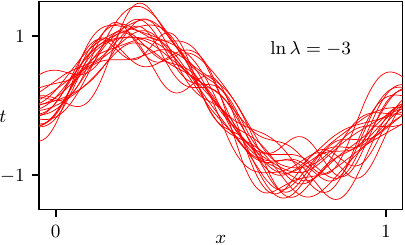
Bias–variance: the same model, many datasets

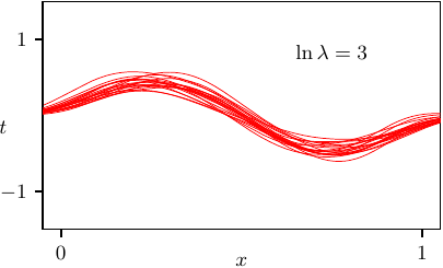
high \(\lambda\) (low capacity) — fits agree → low variance, high bias

low \(\lambda\) (high capacity) — fits scatter → high variance, low bias

Source: Bishop & Bishop (2024), Deep Learning, Fig 4.7 — each red curve is a fit to a different sampled dataset

At one test input the truth is \(h=3\). A rigid model’s fits all land near \(2\); a flexible model’s fits scatter from \(1\) to \(5\) but average exactly \(3\). Which one has the lower expected test error — the biased-but-stable one, or the unbiased-but-wild one?

The decomposition

Let \(h(\vx)=\mathbb{E}[t\given\vx]\) be the best possible prediction, and \(y(\vx;\mathcal D)\) our model trained on a dataset \(\mathcal D\). Averaging over all training sets we could have drawn (\(\mathbb{E}_{\mathcal D}\)):

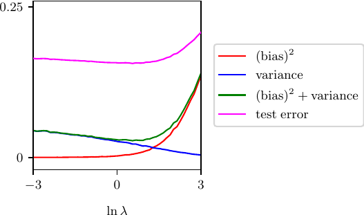
\[ \mathbb{E}_{\mathcal D}\!\big[(y(\vx;\mathcal D)-h(\vx))^2\big] = \underbrace{\big(\mathbb{E}_{\mathcal D}[y]-h\big)^2}_{\text{bias}^2} + \underbrace{\mathbb{E}_{\mathcal D}\!\big[(y-\mathbb{E}_{\mathcal D}[y])^2\big]}_{\text{variance}} \]

  • ↑ capacity: bias² ↓, variance ↑
  • their sum is U-shaped
    • label noise \(\sigma^2\) = expected test error
  • noise is irreducible

Source: Bishop & Bishop (2024), Deep Learning, §4.3, Fig 4.8 · \(y(\vx;\mathcal D)\) = model fit on dataset \(\mathcal D\)

Where the decomposition comes from

Write the error as a deviation from the average model \(\bar y \equiv \mathbb{E}_{\mathcal D}[y(\vx;\mathcal D)]\) (add and subtract \(\bar y\)):

\[ y - h = \big(y - \bar y\big) + \big(\bar y - h\big) \]

Square it and take \(\mathbb{E}_{\mathcal D}\):

\[ \mathbb{E}_{\mathcal D}\big[(y-h)^2\big] = \underbrace{\mathbb{E}_{\mathcal D}\big[(y-\bar y)^2\big]}_{\text{variance}} + \underbrace{(\bar y-h)^2}_{\text{bias}^2} + 2(\bar y-h)\,\underbrace{\mathbb{E}_{\mathcal D}[\,y-\bar y\,]}_{=\,0} \]

The cross term vanishes because \(\mathbb{E}_{\mathcal D}[y-\bar y]=0\) by definition of \(\bar y\) → exactly bias² + variance.

What is \(\mathbb{E}_{\mathcal D}\)? The average over training sets \(\mathcal D\) drawn i.i.d. from \(p(\vx,t)\) — a population (theoretical) expectation, not the empirical distribution of one dataset’s points. We estimate it by retraining on many datasets (the demo used 30); it converges by the law of large numbers. · Bishop §4.3 (cf. PRML §3.2)

Bias and variance on numbers

At one test input \(x_0\) the true value is \(h=3\). We retrain on 4 sampled datasets and read off each model’s prediction at \(x_0\):

\(\mathcal D_1\) \(\mathcal D_2\) \(\mathcal D_3\) \(\mathcal D_4\)
A (rigid) \(1.8\) \(2.2\) \(1.8\) \(2.2\)
B (flexible) \(1.0\) \(3.0\) \(5.0\) \(3.0\)

Model A.\(\bar y=\tfrac{1.8+2.2+1.8+2.2}{4}=2.0\)\(\text{bias}^2=(\bar y-h)^2=(2-3)^2=\mathbf{1.0}\)\(\text{var}=\tfrac{4\times0.2^2}{4}=\mathbf{0.04}\) ④ sum \(=\mathbf{1.04}\)

Model B.\(\bar y=\tfrac{1+3+5+3}{4}=3.0\)\(\text{bias}^2=(3-3)^2=\mathbf{0}\)\(\text{var}=\tfrac{2^2+0+2^2+0}{4}=\mathbf{2.0}\) ④ sum \(=\mathbf{2.0}\)

Predicted right? The biased-but-stable model A wins (\(1.04<2.0\)): B is unbiased, but its variance alone (\(2.0\)) dwarfs A’s whole error. Unbiased ≠ better. (Adding irreducible noise \(\sigma^2\) shifts both totals equally.)

Your turn: a third model

A third model C gives these four fits at the same \(x_0\) (true \(h=3\)):

\[ \hat y \in \{\,2.5,\ 3.5,\ 2.5,\ 3.5\,\} \]

Compute \(\bar y\), \(\text{bias}^2\), variance, and their sum. Is C better or worse than A (\(1.04\)) and B (\(2.0\)) — and which corner of the dartboard (next slide) does it sit in?

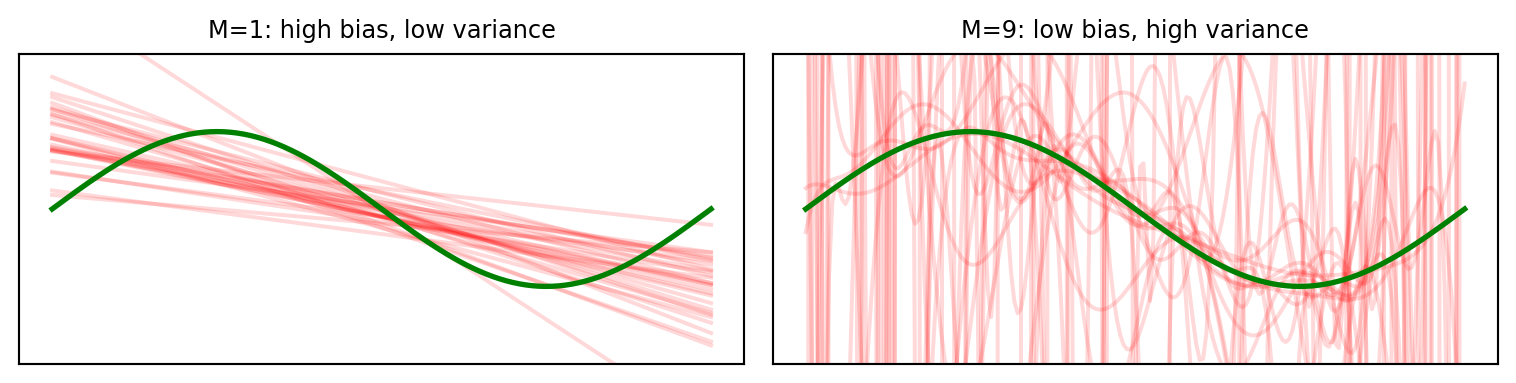
🔬 Demo: variance grows with capacity

import numpy as np, matplotlib.pyplot as plt
rng = np.random.default_rng(0); f = lambda x: np.sin(2*np.pi*x); xs = np.linspace(0, 1, 200)
fig, ax = plt.subplots(1, 2, figsize=(8, 2.1))
for j, (M, ttl) in enumerate([(1, "M=1: high bias, low variance"),
                              (9, "M=9: low bias, high variance")]):
    for _ in range(30):
        x = np.sort(rng.random(10)); t = f(x) + 0.15*rng.standard_normal(10)
        if M == 9: w = np.linalg.solve(np.vander(x, 10), t); p = np.vander(xs, 10) @ w
        else:      w = np.polyfit(x, t, M);                  p = np.polyval(w, xs)
        ax[j].plot(xs, p, "r", alpha=0.15)
    ax[j].plot(xs, f(xs), "g", lw=2)
    ax[j].set_ylim(-2, 2); ax[j].set_title(ttl, fontsize=9); ax[j].set_xticks([]); ax[j].set_yticks([])
plt.tight_layout(); plt.show()

30 models, each fit to a different 10-point sample. M=1 barely moves (low variance); M=9 swings wildly (high variance) — variance is sensitivity to the sample.

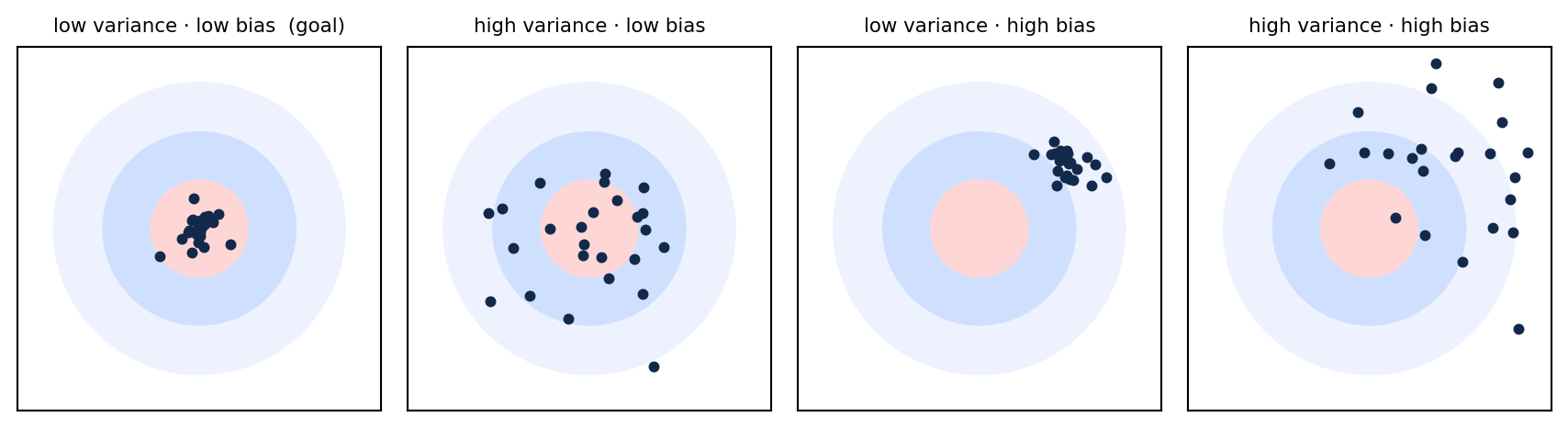
All four corners are possible

Bias and variance are two separate quantities — the trade-off is just one slice (varying capacity at fixed data). On a dartboard: distance to bullseye = bias, spread = variance.

  • low–low = the goal — reachable with more data, a good inductive bias, or the overparameterized regime (double descent)
  • high–high = worst case — wrong model family and unstable (bad features / too little data / poor optimization)

You can get both low — just not by tuning capacity alone

Part 3 · How Much Can a Model Fit?

Computing VC — Step 1: lower bound

A hypothesis class \(\mathcal F\) (the functions the model can represent) shatters points if it can realize every labeling. VC dimension = the largest set \(\mathcal F\) can shatter.

shatter = produce every labeling. So the two steps are not symmetric:

  • ① Lower bound — test \(k\) points: find one set where all \(2^k\) labelings work ⟹ VC \(\ge k\)
  • ② Upper bound — test \(k{+}1\) points: show any such set has ≥ 1 labeling that fails ⟹ VC \(\le k\)

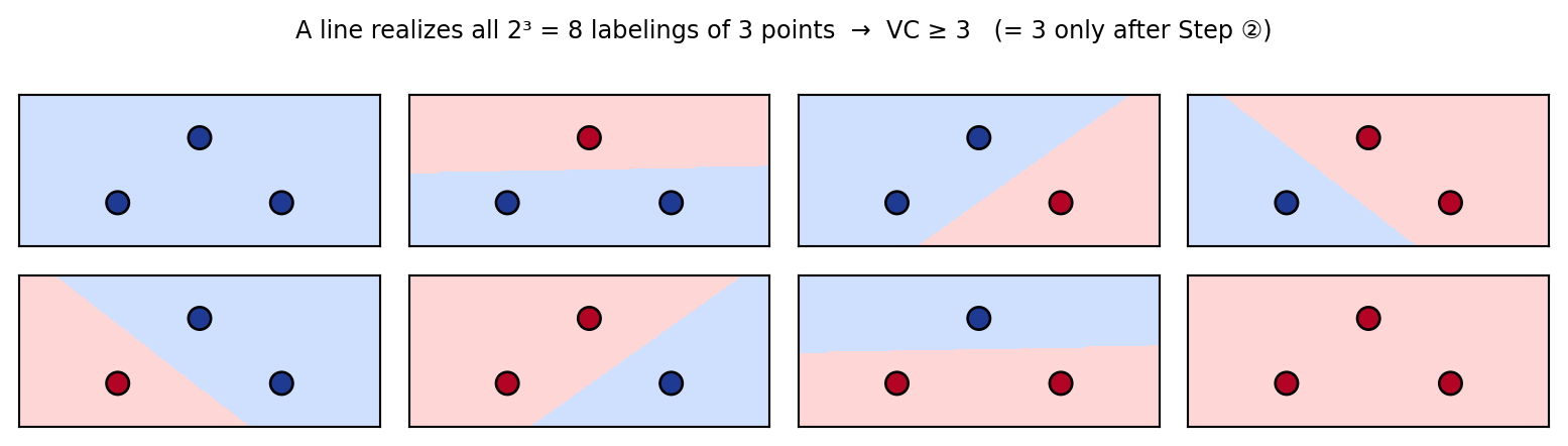
Step ① (\(k=3\)): a line produces all \(2^3=8\) labelings of these 3 points ⟹ VC \(\ge 3\).

VC dimension is from statistical learning theory (Vapnik–Chervonenkis; Shalev-Shwartz & Ben-David, UML) — not covered in Bishop (2024). Figure generated for this course.

We just shattered 3 points. Do you think every set of 4 points can also be shattered by a straight line — or will some 4-point set always have a labeling no line can produce?

Computing VC — Step 2: upper bound

  • Now test \(k{+}1 = 4\) points. Shattering would need all \(2^4=16\) labelings.
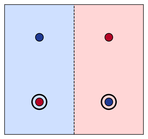
  • We only need one that fails: the XOR labeling — no line separates it (rings = misclassified). So 4 points are not shattered → VC \(< 4\)
  • This fails for any 4 points → with Step ①: VC \(= 3\)

General rule: a linear classifier in \(d\) dimensions has VC dimension \(= d+1\) (= its number of parameters)

To prove VC \(=k\): show some \(k\) points can be shattered (lower bound) and that no \(k{+}1\) points can (upper bound).

Your turn: VC of an interval classifier

A classifier on the real line predicts \(+\) for points inside an interval \([a,b]\) and \(-\) outside.

Use the two-step recipe (lower then upper bound):

  1. Find one set of 2 points where all \(2^2=4\) labelings are achievable ⟹ VC \(\ge 2\).
  2. Show any 3 points \(x_1<x_2<x_3\) have one labeling no interval can produce ⟹ VC \(<3\).

What is the VC dimension — and how does it compare to the number of parameters?

Occam’s razor

Among hypotheses that fit the data equally well, prefer the simplest.

  • “Simple” ≈ low capacity / few effective parameters / small weights
  • Regularization is Occam’s razor written as math (the \(\lambda\norm{\vw}^2\) term, a prior)
  • A simpler model that fits is more likely to generalize

Part 4 · Generalization Bounds & the Modern Puzzle

A bound, in spirit

The classical VC bound plugs the dimension we just computed into a risk bound — with probability \(\ge 1-\delta\):

\[ \underbrace{R(f)}_{\text{true risk}} \;\le\; \underbrace{R_{\text{emp}}(f)}_{\text{train error}} \;+\; \underbrace{O\!\left(\sqrt{\tfrac{d_{\text{VC}}\,\ln N + \ln(1/\delta)}{N}}\right)}_{\text{complexity penalty}} \]

  • the “capacity” is the VC dimension \(d_{\text{VC}}\) from the last two slides
  • more data (\(N\uparrow\)) → smaller gap; more capacity (\(d_{\text{VC}}\uparrow\)) → larger gap
  • it is a PAC guarantee: probably (\(\ge 1-\delta\)) approximately correct (gap small) — next slide

Baseline theory — but with \(d_{\text{VC}}\sim\) #parameters, this bound is vacuous for deep nets

VC bound from statistical learning theory (Vapnik; Shalev-Shwartz & Ben-David) — constants omitted; we only need the shape.

Plug in the line we just analyzed (\(d_{\text{VC}}=3\)), with \(N=1000\) examples and \(\delta=0.05\). Is the complexity penalty closer to 0.015, 0.15, or 1.5?

Worked: when is the bound vacuous?

Penalty \(=\sqrt{\dfrac{d_{\text{VC}}\ln N+\ln(1/\delta)}{N}}\), with \(\delta=0.05\) so \(\ln(1/\delta)=\ln 20\approx 3.0\).

The line (\(d_{\text{VC}}=3,\ N=1000\)): \(\ln 1000\approx 6.91\), so numerator \(=3(6.91)+3.0=23.7\); divide by \(1000\Rightarrow0.0237\); \(\sqrt{\cdot}\approx\mathbf{0.15}\). \(\;\Rightarrow R(f)\le R_{\text{emp}}(f)+0.15\) — a real guarantee (matches the prediction).

A deep net (\(d_{\text{VC}}\sim 10^7,\ N=10^4\)): numerator \(\approx 10^7(9.2)=9.2\times10^7\); divide by \(10^4\Rightarrow 9200\); \(\sqrt{\cdot}\approx\mathbf{96}\). \(\;\Rightarrow R(f)\le R_{\text{emp}}(f)+96\) — but error \(\le 1\) already, so this says nothing: vacuous.

Same formula, two worlds. The penalty is the previous slide’s pillar (\(d_{\text{VC}}\sim\) #parameters) made numeric — and motivates the vacuous-vs-non-vacuous bars coming up.

Your turn: smaller dataset

Re-run the line (\(d_{\text{VC}}=3,\ \delta=0.05\)) but with only \(N=100\) examples instead of \(1000\). Compute the new penalty. Did the guarantee get looser or tighter — and by roughly how much?

The modern puzzle

Classical (VC) theory says huge capacity → overfit. Yet:

  • modern nets have more parameters than data
  • they can even fit random labels (Zhang et al. 2017)
  • …but still generalize on real data

So is classical theory wrong? No — its bounds are just too loose for deep nets.

This motivates the next slides: tools that try to give bounds that actually say something.

Zhang, Bengio, Hardt, Recht & Vinyals (2017), “Understanding deep learning requires rethinking generalization”arXiv:1611.03530

Vacuous vs non-vacuous bounds

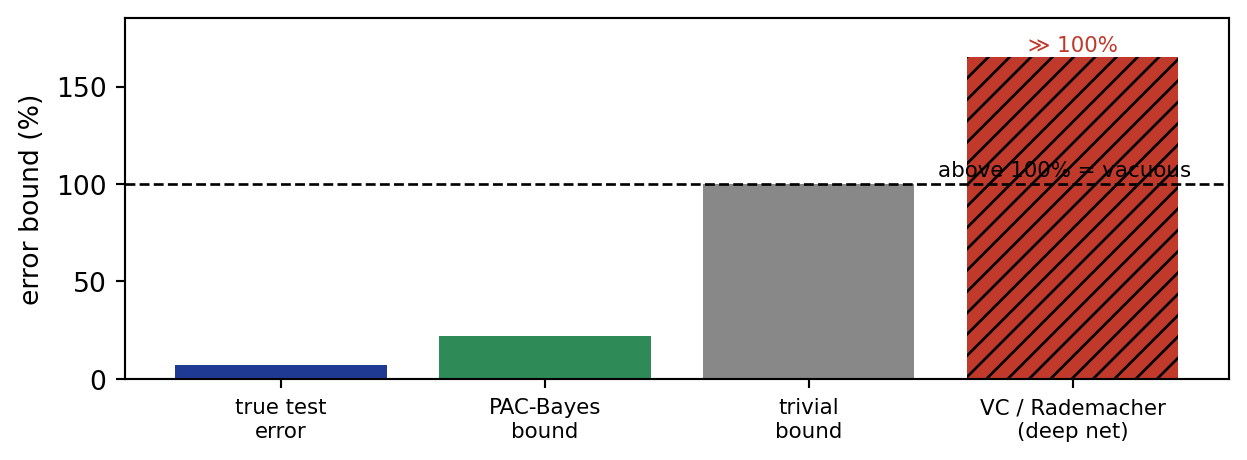
Error always lives in \([0,1]\) — so a bound is only useful if it lands below the trivial 100%.

  • Vacuous = true but says nothing (“error \(\le 500\%\)”) — raw VC / Rademacher for deep nets
  • Non-vacuous = below 100%, a real guarantee (“error \(\le 22\%\)”) — PAC-Bayes (next slide)

A useful bound is a number you’d actually believe — most classical bounds aren’t, for deep nets

PAC learning — the framework

Valiant (1984): from \(N\) samples we can, with probability \(\ge 1-\delta\), find \(f\) whose true risk \(R(f)\le\varepsilon\).

\(\varepsilon\) = target error on the true distribution (= true risk \(R(f)\), not training error) · \(\delta\) = allowed failure probability over the random draw of the training set

  • Probably (\(\ge 1-\delta\)) · Approximately Correct (true error \(R(f)\le\varepsilon\))
  • Sample complexity \(N\sim\dfrac{d_{\text{VC}}+\ln(1/\delta)}{\varepsilon^2}\)polynomial (not exponential) in \(\tfrac1\varepsilon,\tfrac1\delta,d_{\text{VC}}\)
  • richer class (\(d_{\text{VC}}\uparrow\)) ⟹ need more data for the same \(\varepsilon,\delta\)
  • the bound on the previous slide is a PAC statement: it certifies \(R(f)\) using \(R_{\text{emp}}(f)\) + complexity
  • distribution-free — holds for any \(p(\vx,t)\) (its strength and its weakness)

PAC is the language of generalization guarantees — but VC-based PAC bounds are vacuous for deep nets

Valiant (1984), “A theory of the learnable” (CACM)

Rademacher complexity — data-dependent capacity

How well can the hypothesis class \(\mathcal F\) fit random \(\pm1\) labels on your own sample?

\[ \mathfrak{R}_N(\mathcal F) = \mathbb{E}_{\boldsymbol\sigma}\Big[\,\sup_{f\in\mathcal F}\tfrac1N\textstyle\sum_{n=1}^N \sigma_n\,f(\vx_n)\Big],\quad \sigma_n\in\{-1,+1\} \]

\[ R(f) \le R_{\text{emp}}(f) + 2\,\mathfrak{R}_N(\mathcal F) + O\!\big(\sqrt{\tfrac{\ln(1/\delta)}{N}}\big) \]

  • data-dependent (uses your \(\vx_n\)) and usually tighter than VC
  • Zhang 2017: a deep net fits random labels ⟹ unconstrained \(\mathfrak{R}_N\) is maximal → vacuous
  • …but norm-/margin-controlled \(\mathfrak{R}_N\) gives meaningful bounds (Bartlett et al. 2017)

The fix: measure capacity by norm / margin, not parameter count

norm-/margin-controlled = measure \(\mathfrak{R}_N\) only over the subset SGD actually reaches — small weight-norm \(\{\|\vw\|\le B\}\) and large margin \(\gamma\) (distance of correct points from the boundary). It then grows with the norm, not #parameters. · Bartlett & Mendelson (2002) · margin bounds: Bartlett, Foster & Telgarsky (2017)

PAC-Bayes — non-vacuous bounds for deep nets

Bound the average risk over a posterior \(Q\) relative to a prior \(P\) — with prob \(\ge 1-\delta\):

\[ \mathbb{E}_{f\sim Q}\!\big[R(f)\big] \;\le\; \mathbb{E}_{f\sim Q}\!\big[R_{\text{emp}}(f)\big] + \sqrt{\frac{\mathrm{KL}(Q\,\|\,P) + \ln(N/\delta)}{2N}} \]

  • complexity = \(\mathrm{KL}(Q\,\|\,P)\) — small when the solution is simple / flat relative to the prior (recall KL from Lecture 2!)
  • it adapts to the learned solution, not the worst case in \(\mathcal F\)
  • Dziugaite & Roy (2017): optimizing this bound gave the first non-vacuous bound for a real deep net
  • Lotfi et al. (2022): compression-based PAC-Bayes bounds tight enough to explain generalization — big models compress far more than expected (Occam’s razor made quantitative)

The most successful capacity-style explanation of deep generalization so far

McAllester (1999) · Dziugaite & Roy (2017) · Lotfi, Finzi, Goldblum, Wilson et al., PAC-Bayes compression bounds (2022)

From Vapnik’s theory to deep networks

It still applies — but is vacuous

  • A net with \(W\) weights has finite VC dim (e.g. \(\sim O(W\log W)\))
  • For modern nets the bound is astronomically large → true but useless
  • So classical VC reveals the paradox rather than resolving it

Vapnik’s deeper ideas are the bridge

  • Margin (his own SVM idea): SGD finds large-margin solutions
  • Implicit regularization: SGD prefers small-norm / flat minima → effective capacity \(\ll W\)
  • Neural tangent kernel: very wide nets \(\approx\) kernel machines → back to classical theory
  • Double descent: extends the capacity curve past interpolation (next two slides)

Statistical learning theory gives the vocabulary and the questions (capacity, margin, generalization) — it is the baseline you measure deep learning against, not yet a full theory of it

Vapnik (1995), The Nature of Statistical Learning Theory · Bartlett et al. margin bounds (2017) · Jacot et al. NTK (2018) · Zhang et al. rethinking generalization (2017)

Double descent

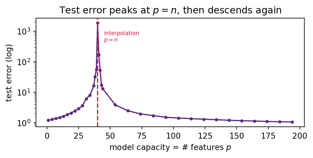
The bias–variance U-curve is only half the picture. Push capacity past the interpolation threshold (\(P \approx N\), zero training error) and test error rises to a peak, then falls again.

  • classical regime (\(P<N\)): the familiar U-curve
  • interpolation (\(P\approx N\)): one exact fit → wild, high-variance
  • modern regime (\(P\gg N\)): many exact fits → SGD picks a smooth, min-norm one

Pillar: “bigger than the data” is not automatically worse. Past interpolation, implicit regularization chooses among the many zero-error solutions — resolving the L0/L4 puzzle.

Belkin et al. (2019) · Nakkiran et al., Deep Double Descent (2019)

🔬 Demo: the double descent curve

import numpy as np, matplotlib.pyplot as plt
rng = np.random.default_rng(0)
d, n, sigma = 200, 40, 0.5                       # ambient dim, train size, noise
beta = rng.normal(0, 1, d) / np.sqrt(d)
def data(m): X = rng.normal(0,1,(m,d)); return X, X @ beta + sigma*rng.normal(size=m)
Xte, yte = data(2000)

ps = np.unique(np.r_[np.arange(1,n,3), np.arange(n-3,n+4), np.arange(n+4,d+1,10)])
err = np.zeros(len(ps))
for _ in range(20):                              # average test risk over datasets
    Xtr, ytr = data(n)
    for j, p in enumerate(ps):
        w = np.linalg.pinv(Xtr[:,:p]) @ ytr      # min-norm least squares
        err[j] += np.mean((Xte[:,:p] @ w - yte)**2)
err /= 20

plt.figure(figsize=(5.6,2.9))
plt.semilogy(ps, err, "o-", ms=3, color="#5d2c80")
plt.axvline(n, ls="--", c="crimson"); plt.text(n+5, err.max()*0.25, "interpolation\n$p=n$", fontsize=7, c="crimson")
plt.xlabel("model capacity = # features $p$"); plt.ylabel("test error (log)")
plt.title("Test error peaks at $p=n$, then descends again"); plt.tight_layout(); plt.show()

The Lottery Ticket Hypothesis

The flip side of overparameterization (Frankle & Carbin, 2019):

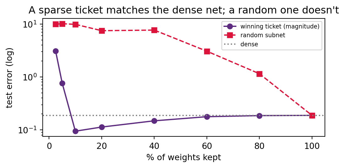
A dense, randomly-initialized network contains a sparse subnetwork — a “winning ticket” — that, trained from the same initialization, matches the full network.

Found by iterative magnitude pruning: train → prune smallest weights → rewind survivors to their original init → retrain.

Pillar: overparameterization may help mainly by giving SGD many subnetworks to try — a lucky, well-initialized small one was enough all along. (The same init is essential — a random subnet of equal size fails.)

Frankle & Carbin, The Lottery Ticket Hypothesis (2019)

🔬 Demo: a winning ticket vs a random subnet

import numpy as np, matplotlib.pyplot as plt
rng = np.random.default_rng(0)
P, n, s = 200, 400, 20                                    # P features; true support = s
beta = np.zeros(P); supp = rng.choice(P, s, replace=False); beta[supp] = rng.normal(0,1,s)
def data(m): X = rng.normal(0,1,(m,P)); return X, X @ beta + 0.3*rng.normal(size=m)
Xtr, ytr = data(n); Xte, yte = data(4000)
w = np.linalg.lstsq(Xtr, ytr, rcond=None)[0]             # dense fit
order = np.argsort(np.abs(w))[::-1]                       # rank by magnitude

ks = [5,10,20,40,80,120,160,200]; e_tic, e_rnd = [], []
for k in ks:
    t = order[:k]; e_tic.append(np.mean((Xte[:,t] @ np.linalg.lstsq(Xtr[:,t],ytr,rcond=None)[0] - yte)**2))
    r = rng.choice(P,k,replace=False); e_rnd.append(np.mean((Xte[:,r] @ np.linalg.lstsq(Xtr[:,r],ytr,rcond=None)[0] - yte)**2))

plt.figure(figsize=(5.6,2.9))
plt.semilogy([k/P*100 for k in ks], e_tic, "o-", color="#5d2c80", label="winning ticket (magnitude)")
plt.semilogy([k/P*100 for k in ks], e_rnd, "s--", color="crimson", label="random subnet")
plt.axhline(np.mean((Xte@w-yte)**2), ls=":", c="gray", label="dense")
plt.xlabel("% of weights kept"); plt.ylabel("test error (log)"); plt.legend(fontsize=7)
plt.title("A sparse ticket matches the dense net; a random one doesn't"); plt.tight_layout(); plt.show()
Summary

  1. We minimize empirical risk, but care about true risk — the gap is everything
  2. Capacity trades bias↓ vs variance↑; balance it (not “as big as possible”). Occam’s razor = prefer simple → regularization
  3. Measuring capacity: VC (vacuous for deep nets) → norm/margin (Rademacher) & PAC-Bayes give the first non-vacuous bounds
  4. Classical theory is the baseline; deep nets generalize via implicit regularization (margin / flat minima) + data + architecture — still partly open
  5. Double descent & the lottery ticket: past interpolation, more capacity can help — and a tiny well-initialized subnetwork was often enough all along

Something to think about: a model with \(10^9\) parameters trained on \(10^4\) images reaches 0 training error. Classical theory is alarmed — give two reasons it might still generalize.

📌 Read before next class

Bishop & Bishop (2024), Chapter 6Deep Neural Networks

We finally learn the features instead of choosing them: multilayer perceptrons, activation functions, and the universal approximation theorem.

Figures from Bishop & Bishop, Deep Learning: Foundations and Concepts (2024), Chapter 4 — https://www.bishopbook.com/

⌂ Home