Lecture 8 — Regularization

Deep Learning · Session 8

Kasemsit Teeyapan

Department of Computer Engineering, Chiang Mai University

Today

1. Regularization = injecting prior knowledge to control effective capacity
2. Weight decay (L2) — and L1 sparsity
3. Early stopping — read it off the validation curve
4. Dropout & data augmentation
5. Normalization and residual connections — make very deep nets trainable

Reference: Bishop & Bishop (2024), Chapter 9 — Regularization

เปิดคาบ: ตอนนี้เทรน deep net ได้แล้ว (L6 GD + L7 backprop) แต่มันจะ overfit (L0/L4) คาบนี้ = วิธีกัน overfitting + เทคนิคที่ทำให้ net ลึกมาก ๆ เทรนได้ (norm, residual — เชื่อม vanishing gradient จาก L7) ~1.5 นาที

Recap → why regularize

• L4: high capacity → variance / overfitting
• deep nets have more parameters than data
• yet we want big models (they generalize well — if controlled)

Regularization = anything that reduces the gap \(R(f)-R_{\text{emp}}(f)\) without just shrinking the model:

• a prior on weights, noise, invariances, ensembling…

We don’t make the model smaller — we constrain how it fits, so capacity is spent on signal, not noise

เชื่อม L4: capacity สูง→variance/overfit; deep net พารามิเตอร์มากกว่าข้อมูล แต่เราอยากได้โมเดลใหญ่ (generalize ดีถ้าคุมเป็น) regularization = อะไรก็ตามที่ลด generalization gap โดยไม่ต้องย่อโมเดล (prior, noise, invariance, ensemble) ย้ำ pillar: ไม่ทำโมเดลเล็กลง แต่ “คุมวิธี fit” ให้ capacity ไปกับ signal ไม่ใช่ noise ~2 นาที

Part 1 · Inductive Bias

No free lunch — you must assume something

No free lunch theorem: averaged over all possible problems, every learner is equally (un)good. Generalization is only possible because real problems have structure.

Regularization = the assumptions we build in:

• functions are smooth (small weights) → weight decay
• predictions are invariant to small changes (shift, rotation) → augmentation, conv
• simpler explanations are preferred → Occam’s razor (L4)

Every regularizer encodes a belief about the world — choosing it well is machine-learning expertise

No free lunch: เฉลี่ยเหนือ “ทุกปัญหาที่เป็นไปได้” ทุก learner เก่งเท่ากันหมด (=ไม่มีอะไรดีกว่าโดยสากล) → generalize ได้เพราะปัญหาจริงมีโครงสร้าง regularization = สมมติฐานที่เราใส่: ฟังก์ชันเรียบ (weights เล็ก→weight decay), invariant ต่อการเปลี่ยนเล็กน้อย (augmentation/conv), เลือกอันง่ายกว่า (Occam, L4) ย้ำ pillar: regularizer ทุกตัว = ความเชื่อเกี่ยวกับโลก เลือกเป็น=ความเชี่ยวชาญ ML ~2 นาที

Part 2 · Weight Decay

A two-point fit

One weight, no bias: predict \(t \approx w\,x\) from two points \((x,t)=(1,2)\) and \((2,2)\).

• plain least squares minimizes \(E(w)=\tfrac12\sum_n (t_n-w x_n)^2\)
• its solution is \(w^\star=\dfrac{\sum_n x_n t_n}{\sum_n x_n^2}=\dfrac{6}{5}=1.2\)

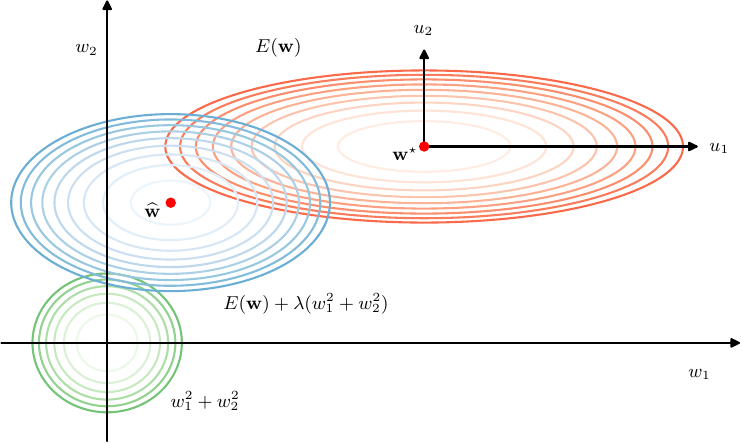
Now add a penalty \(\tfrac{\lambda}{2}w^2\) that dislikes large weights.

Before any algebra: when we switch on the penalty \(\lambda>0\), does the fitted \(w\) move toward 0, away from 0, or stay at 1.2? Why?

ตั้งโจทย์ของจริงเล็ก ๆ ก่อนทฤษฎี: w เดียว ไม่มี bias จุด (1,2),(2,2) least squares ได้ w*=6/5=1.2 ให้ นศ เดา (30–60 วิ) ก่อนพิสูจน์: เปิด penalty λ/2 w² แล้ว w จะขยับเข้าหา 0 / ออกจาก 0 / อยู่ที่เดิม? อย่าเพิ่งเฉลย เก็บไว้เทียบกับ worked example หลัง MAP ~1.5 นาที

L2 = a Gaussian prior on weights

\[ \widetilde E(\vw) = E(\vw) + \frac{\lambda}{2}\,\norm{\vw}^2 \]

• shrinks weights toward 0 → smoother functions
• exactly the ridge / MAP view from Lecture 2 (\(\lambda=\alpha/\beta\))
• \(\lambda\) trades fit vs simplicity — tune on validation
• L1 (\(\lambda\sum|w_i|\)) instead → drives weights to exactly 0 (sparsity)

Source: Bishop & Bishop (2024), Deep Learning, Fig 9.3 — error contours (red) meet the regularizer

weight decay = เพิ่ม λ/2‖w‖² → ดึง weights เข้าใกล้ 0 → ฟังก์ชันเรียบขึ้น นี่คือ ridge/MAP จาก L2 เป๊ะ (Gaussian prior, λ=α/β) รูป: contour error (แดง) ชนกับ contour ของ regularizer → จุด optimum ขยับเข้าหา 0 L1 (Σ|w|) แทน → ดัน weight เป็น 0 จริง (sparsity, มุมของ diamond) λ จูนบน validation ~2.5 นาที

Where weight decay comes from (MAP)

Maximum a posteriori: maximize \(p(\vw\given\mathcal D)\propto p(\mathcal D\given\vw)\,p(\vw)\).

• Gaussian prior \(p(\vw)=\mathcal N(0,\alpha^{-1}I)\propto e^{-\frac{\alpha}{2}\norm{\vw}^2}\)
• Gaussian likelihood \(\propto e^{-\frac{\beta}{2}\sum_n (y_n-t_n)^2}\)

Take \(-\ln\) of the posterior:

\[-\ln p(\vw\given\mathcal D) = \tfrac{\beta}{2}\sum_n(y_n-t_n)^2 + \tfrac{\alpha}{2}\norm{\vw}^2 + \text{const}\]

\[\propto\; E(\vw) + \tfrac{\lambda}{2}\norm{\vw}^2,\quad \lambda=\tfrac{\alpha}{\beta}\]

Pillar: weight decay is MAP estimation with a Gaussian prior. A stronger belief that weights are small (larger \(\alpha\)) = larger \(\lambda\) = more shrinkage. The regularizer is a prior (L2).

derivation weight decay = MAP (เติมรากฐานให้สไลด์ที่แล้วที่กล่าวลอย ๆ): MAP = maximize posterior p(w|D) ∝ p(D|w)p(w) ใส่ Gaussian prior p(w)=N(0,α⁻¹I) ∝ exp(-α/2‖w‖²) และ Gaussian likelihood ∝ exp(-β/2 Σ(y-t)²) เอา -ln posterior: = β/2 Σ(y-t)² + α/2‖w‖² + const → หารด้วย β ได้ E(w) + λ/2‖w‖² โดย λ=α/β เป๊ะ! ย้ำ pillar: weight decay “คือ” MAP ที่มี Gaussian prior — เชื่อว่า weight เล็ก (α ใหญ่) → λ ใหญ่ → shrink มาก regularizer = prior (เชื่อม L2 Bayesian) ให้ นศ เห็นว่า L2 ไม่ใช่ heuristic แต่มาจากความน่าจะเป็น ~2.5 นาที

Solving the two-point fit

Setting \(\dfrac{d}{dw}\!\left[E(w)+\tfrac{\lambda}{2}w^2\right]=0\) gives the ridge solution \[ w^\star=\frac{\sum_n x_n t_n}{\sum_n x_n^2 + \lambda}=\frac{6}{5+\lambda}. \]

With \(\sum x_n t_n = 6\) and \(\sum x_n^2 = 5\):

• \(\lambda=0\):  \(w^\star = 6/5 = \mathbf{1.2}\) (plain least squares)
• \(\lambda=1\):  \(w^\star = 6/6 = \mathbf{1.0}\)
• \(\lambda=5\):  \(w^\star = 6/10 = \mathbf{0.6}\)

The penalty adds to the denominator, so \(w^\star\) shrinks toward 0 — never past it. Did your prediction match?

Same two points, but crank the penalty to \(\lambda=7\). Compute \(w^\star\). How much of the unregularized \(1.2\) is left?

worked: หา ridge solution จาก d/dw[E+λ/2 w²]=0 → w=Σxt/(Σx²+λ)=6/(5+λ) แทนค่า λ=0→1.2, λ=1→1.0, λ=5→0.6 เน้น: λ ไปอยู่ “ตัวส่วน” → ดึง w เข้าหา 0 (ไม่เลยศูนย์) ปิด loop: ตรงกับที่เดาไหม (เข้าหา 0) solo เฉลย: λ=7 → w=6/(5+7)=6/12=0.5 เหลือครึ่งเดียวของ 1.2 (พอดี 0.5/1.2≈42%) ให้ นศ ลองเอง ~2 นาที

Part 3 · Early Stopping

Stop at the validation minimum

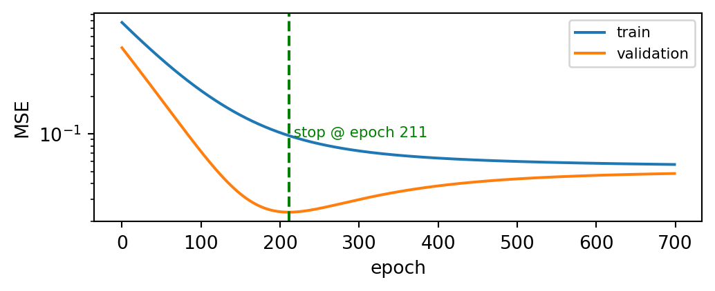
Training error keeps dropping; validation error turns back up when the model starts fitting noise.

We fit 15 Gaussian bumps to 15 noisy points by gradient descent for 700 epochs. Training MSE will fall the whole way. What does the validation MSE do — fall too, flatten, or fall-then-rise? Where would you stop?

import numpy as np, matplotlib.pyplot as plt
rng = np.random.default_rng(0)
xt = np.linspace(0, 1, 15); tt = np.sin(2*np.pi*xt) + 0.35*rng.standard_normal(15)
xv = np.linspace(0, 1, 200); tv = np.sin(2*np.pi*xv)             # clean held-out truth
mu = np.linspace(0, 1, 15); s = 0.12
feat = lambda x: np.exp(-0.5*((x[:, None]-mu)/s)**2)
P, Pv = feat(xt), feat(xv); w = np.zeros(15); tr, va = [], []
for _ in range(700):                                            # gradient descent
    w -= 0.01 * P.T @ (P @ w - tt) / len(xt)
    tr.append(np.mean((P@w-tt)**2)); va.append(np.mean((Pv@w-tv)**2))
best = int(np.argmin(va))
plt.figure(figsize=(5.5, 2.3))
plt.plot(tr, label="train"); plt.plot(va, label="validation")
plt.axvline(best, color="g", ls="--"); plt.text(best, va[best]*4, f" stop @ epoch {best}", color="g", fontsize=8)
plt.yscale("log"); plt.xlabel("epoch"); plt.ylabel("MSE"); plt.legend(fontsize=8); plt.tight_layout(); plt.show()

Train MSE → 0, but validation bottoms out then rises. Early stopping = keep the weights at that minimum.

predict ก่อนรัน (30 วิ): val MSE จะลด/แบน/ลงแล้วเด้งขึ้น? จะหยุดตรงไหน? แล้วรันสด: train MSE ลดเรื่อย ๆ ลง 0 (overfit) แต่ validation ลดแล้ว “เด้งกลับ” เมื่อเริ่ม fit noise เส้นเขียว=จุดต่ำสุดของ val → early stopping = หยุด/เก็บ weights ที่จุดนั้น (เชื่อม U-curve L0/L4) เกร็ด: early stopping มีผลคล้าย weight decay (จำกัดว่า weights ขยับจาก 0 ได้ไกลแค่ไหน) ~2.5 นาที

Part 4 · Dropout & Augmentation

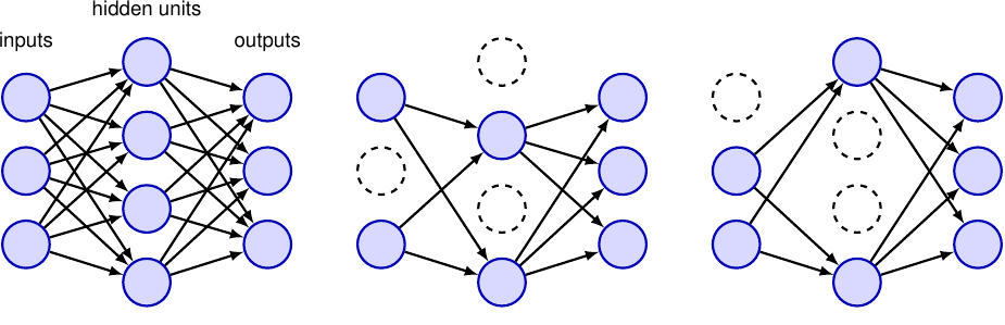
Dropout: train an ensemble for free

• each step, keep each unit with prob \(p\) (drop it with prob \(1-p\))
• every mini-batch trains a different thinned network
• units can’t co-adapt → robust features
• at test: keep all units, scale by \(p\) ≈ averaging the ensemble

A unit normally outputs \(a=4\). During training it is kept only \(p=\tfrac14\) of the time. At test time we leave it always on (output \(4\)). To keep the next layer seeing the same average input as during training, what should we multiply the test output by?

Dropout ≈ training & averaging exponentially many sub-networks — strong, cheap regularization

Source: Bishop & Bishop (2024), Deep Learning, Fig 9.17 · Srivastava, Hinton, Krizhevsky, Sutskever & Salakhutdinov (2014), JMLR

dropout: แต่ละก้าวสุ่ม “ลบ” หน่วยทิ้ง (ความน่าจะเป็น p) → ทุก mini-batch เทรน net ที่ “ผอม” คนละแบบ หน่วยพึ่งพากันไม่ได้ (co-adapt) → feature ทนทาน ตอน test: ใช้ทุกหน่วย คูณ p ≈ เฉลี่ย ensemble ย้ำ pillar: dropout ≈ เทรน+เฉลี่ย sub-network จำนวนมหาศาล = regularization แรงและถูก (paper assign: Srivastava 2014) อย่าลืมเฉลย predict ในสไลด์ถัดไป ~2.5 นาที

Why scale by \(p\) at test

During training a unit is on with prob \(p\), off otherwise, so the next layer sees it with expected value \[ \E[\text{output}] = p\cdot a + (1-p)\cdot 0 = p\,a. \]

Unit value \(a=4\), keep prob \(p=\tfrac14\).

• Train (averaged over masks): \(\E[\text{output}] = \tfrac14 \cdot 4 = \mathbf{1}\)
• Test, naively always on: output \(=4\) — 4× too big!
• Fix: multiply by \(p\) → \(4\times\tfrac14 = \mathbf{1}\) ✓ matches training

So the test-time scale factor is exactly \(p\). Did your prediction match?

A unit outputs \(a=5\) and is kept with prob \(p=0.4\). (a) What expected value does the next layer see during training? (b) What must we multiply the always-on test output by, and what value does it give?

worked เติมรากฐานให้ “scale by p”: ตอนเทรน หน่วยติดด้วยความน่าจะเป็น p → ค่าคาดหวัง = p·a + (1-p)·0 = p·a แทน a=4, p=1/4 → train E=1 แต่ test ถ้าเปิดตลอด = 4 (ใหญ่ไป 4 เท่า) แก้: คูณ p → 4·1/4=1 พอดี ปิด loop ตรงกับ predict (คูณ p=1/4) solo เฉลย: a=5, p=0.4 → (a) train E = 0.4·5 = 2 (b) คูณด้วย p=0.4 → 5·0.4 = 2 พอดี ~2 นาที

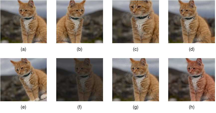
Data augmentation encodes invariance

• expand the data with label-preserving transforms (flip, crop, color, rotate)
• teaches the model what to be invariant to
• a free way to inject domain knowledge — often the single biggest win in vision

The cat is still a cat after a flip — augmentation builds that invariance into the training set.

Source: Bishop & Bishop (2024), Deep Learning, Fig 9.1

data augmentation: เพิ่มข้อมูลด้วยการแปลงที่ “ไม่เปลี่ยน label” (พลิก/ครอป/สี/หมุน) → สอนโมเดลว่าควร invariant ต่ออะไร เป็นวิธีใส่ความรู้โดเมนฟรี ๆ มักเป็นตัวช่วยที่ได้ผลที่สุดใน vision รูป: แมวพลิก/ปรับแสง ก็ยังเป็นแมว ~2 นาที

Part 5 · Making Deep Nets Trainable

Normalization stabilizes training

Normalize each layer’s activations to zero mean / unit variance (then rescale with learned \(\gamma,\beta\)):

• Batch norm: normalize across the mini-batch — speeds up training, mild regularizer
• Layer norm: normalize across features of one example — used in Transformers

• keeps activations in a good range → larger learning rates, less sensitivity to init
• reduces internal “moving target” between layers

Normalization is why we deferred it from Lecture 6 — it’s a practical lever for both optimization and regularization.

Bishop §7.4 (batch / layer normalization)

normalization: ปรับ activation แต่ละชั้นให้ mean 0 var 1 แล้ว rescale ด้วย γ,β ที่เรียนได้ batch norm=normalize ข้าม mini-batch (เร่งเทรน + regularize เบา ๆ), layer norm=normalize ข้าม feature ของตัวอย่างเดียว (ใช้ใน Transformer) ผล: activation อยู่ช่วงดี → ใช้ lr ใหญ่ขึ้น, ไวต่อ init น้อยลง, ลด “เป้าเคลื่อน” ระหว่างชั้น (เลื่อนมาจาก L6 เพราะช่วยทั้ง optimization และ regularization) ~2.5 นาที

Normalizing a mini-batch

For activations \(\{a_1,\dots,a_N\}\): subtract the mean, divide by the std, then rescale: \[ \hat a_i = \frac{a_i-\mu}{\sigma},\qquad y_i = \gamma\,\hat a_i + \beta. \]

A batch of activations is \(\{3,3,7,7\}\). After subtracting the mean and dividing by the standard deviation, what is the mean and variance of the \(\hat a_i\)? (No calculator needed for the answer.)

Batch \(\{3,3,7,7\}\), with learned \(\gamma=2,\ \beta=1\):

• mean \(\mu = \tfrac{3+3+7+7}{4}=5\)
• variance \(\sigma^2 = \tfrac{(-2)^2+(-2)^2+2^2+2^2}{4}=4,\quad \sigma=2\)
• normalized \(\hat a = \bigl[\tfrac{3-5}{2},\dots\bigr]=[-1,-1,1,1]\) → mean \(0\), var \(1\) ✓
• rescaled \(y=\gamma\hat a+\beta = [-1,-1,3,3]\)

Batch \(\{2,2,8,8\}\) with \(\gamma=4,\ \beta=2\). Find \(\mu,\sigma\), the normalized \(\hat a\), and the output \(y\).

worked normalization บนตัวเลขจริง: batch {3,3,7,7} → μ=5, σ²=((-2)²·2+2²·2)/4=4, σ=2, x̂=[-1,-1,1,1] (mean0 var1 เสมอ — ตอบ predict) แล้ว rescale γ=2,β=1 → y=[-1,-1,3,3] เน้น: γ,β เรียนได้ ทำให้ net “ถอน” normalization ได้ถ้าจำเป็น solo เฉลย: {2,2,8,8} → μ=5, σ²=((-3)²·2+3²·2)/4=9, σ=3, x̂=[-1,-1,1,1], y=4·x̂+2=[-2,-2,6,6] ~2 นาที

Residual connections fix vanishing gradients

\[ \mathbf z = \vx + F(\vx) \]

• a layer learns a residual, not the whole map
• the skip path lets gradients flow straight back → no vanishing (L7!)
• enables networks hundreds of layers deep (ResNet)

The simplest fix to L7’s vanishing-gradient problem — and the reason modern nets can be so deep

Source: Bishop & Bishop (2024), Deep Learning, Fig 9.13 · He et al., ResNet (2016)

residual connection: z = x + F(x) — ชั้นเรียน “ส่วนต่าง” (residual) ไม่ใช่ทั้งฟังก์ชัน เส้นลัด (skip) ให้ gradient ไหลย้อนตรง ๆ → ไม่ vanishing (แก้ปัญหา L7!) → เทรน net ลึกหลายร้อยชั้นได้ (ResNet, He 2016 = paper ใน reading list) ย้ำ pillar: นี่คือทางแก้ vanishing gradient ที่ง่ายสุด และเป็นเหตุผลที่ net สมัยใหม่ลึกได้ขนาดนี้ ~2.5 นาที

How the skip path saves the gradient

Backprop multiplies one local factor per layer (L7). Say every layer scales the gradient by 0.5.

Through a plain 10-layer stack, the gradient reaching layer 1 is multiplied by \(0.5\) ten times. A residual block is \(z=x+F(x)\), so its local factor is \(1+F'\) instead of just \(F'\). Which gradient survives — and roughly how big is each?

Plain: factor \(= 0.5^{10} = 0.00098\) — the gradient is ~1000× smaller at layer 1 → it vanishes.

Residual: the skip adds 1 to each factor, so each layer multiplies by \(1+0.5=1.5\): \[ 1.5^{10} \approx 57. \] Even ignoring \(F\), the skip alone gives a factor of \(1^{10}=1\) — the gradient can’t vanish. That’s why ResNets train at hundreds of layers.

Make the stack 20 layers deep, same \(0.5\) per layer. (a) Plain factor \(0.5^{20}=?\) (order of magnitude). (b) What is the skip-path-only factor? Which network is still trainable?

worked เชื่อม L7 vanishing gradient เป็นตัวเลข: backprop คูณ local factor ทีละชั้น สมมติชั้นละ 0.5 plain 10 ชั้น: 0.5¹⁰=0.00098 → เล็กลง ~1000 เท่า = vanish residual: skip บวก 1 ทุกชั้น → factor 1+0.5=1.5 → 1.5¹⁰≈57 และต่อให้ F=0 เส้น skip ล้วน ๆ ก็ให้ 1¹⁰=1 (ไม่มีวันหาย) ปิด loop ตรงกับ predict (residual รอด) solo เฉลย: (a) 0.5²⁰≈9.5×10⁻⁷ (เล็กมาก vanish หนัก) (b) skip-only = 1²⁰ = 1 → residual เทรนได้, plain ตายสนิท ~2 นาที

Summary

1. Regularization = inject prior knowledge to spend capacity on signal, not noise (no free lunch)
2. Weight decay (= L2 / Gaussian prior, L2 lecture); L1 → sparsity
3. Early stopping (validation minimum); dropout (ensemble); augmentation (invariance)
4. Normalization + residual connections make very deep nets trainable (residuals fix vanishing gradients)

Something to think about: “inverted dropout” skips the test-time scaling and instead divides by \(p\) during training. Show this leaves the test network unchanged — and explain why frameworks prefer it. (Hint: compare the expected input to the next layer in both schemes.)

สรุป 4 ข้อ โจทย์คิดต่อ (ต่อยอดจาก worked dropout): inverted dropout ไม่สเกลตอน test แต่ “หารด้วย p ตอนเทรน” แทน → ตอนเทรน E=p·a·(1/p)=a เท่ากับ test ที่เปิดเต็ม → test net ไม่ต้องแก้อะไรเลย (เร็วกว่า, deploy ง่าย) เป็นเหตุผลที่ framework ส่วนใหญ่ใช้ inverted dropout เชื่อมไป CNN ~1.5 นาที

📌 Read before next class

Bishop & Bishop (2024), Chapter 10 — Convolutional Networks

Our first specialized architecture: parameter sharing and convolution bake image invariances right into the network.

Figures from Bishop & Bishop, Deep Learning: Foundations and Concepts (2024), Chapter 9 — https://www.bishopbook.com/

สั่งอ่าน Ch10 (Convolutional Networks) ล่วงหน้า เกริ่น: สถาปัตยกรรมเฉพาะทางตัวแรก — parameter sharing + convolution ฝัง invariance ของภาพเข้าไปในโครงสร้างเลย (เชื่อม inductive bias วันนี้) อาจมี reading quiz ~30 วินาที