\( \newcommand{\vw}{\mathbf{w}} \newcommand{\vx}{\mathbf{x}} \newcommand{\vt}{\mathbf{t}} \newcommand{\vy}{\mathbf{y}} \newcommand{\vz}{\mathbf{z}} \newcommand{\vq}{\mathbf{q}} \newcommand{\vk}{\mathbf{k}} \newcommand{\vv}{\mathbf{v}} \newcommand{\vc}{\mathbf{c}} \newcommand{\vp}{\mathbf{p}} \newcommand{\vh}{\mathbf{h}} \newcommand{\vmu}{\boldsymbol{\mu}} \newcommand{\vsigma}{\boldsymbol{\sigma}} \newcommand{\vepsilon}{\boldsymbol{\epsilon}} \newcommand{\R}{\mathbb{R}} \newcommand{\E}{\mathbb{E}} \newcommand{\norm}[1]{\lVert #1 \rVert} \newcommand{\given}{\,\vert\,} \)

Lecture 13 — Language Models: GPT & BERT

Deep Learning · Session 13

Kasemsit Teeyapan

Department of Computer Engineering, Chiang Mai University

Today

  1. What a language model is: an autoregressive distribution over token sequences
  2. Tokenization (text → tokens) and word embeddings (tokens → vectors)
  3. Two training objectives: GPT (causal/next-token) vs BERT (masked)
  4. Decoding strategies: greedy, beam, temperature, top-k, top-p
  5. Pretrain → fine-tune → in-context learning — how one model serves many tasks

Reference: Bishop & Bishop (2024), §12.2–12.3 — Natural Language & Transformer Language Models

Recap → what is a language model?

L10 gave us the transformer. A language model uses it to model a probability distribution over token sequences:

\[p(y_1,\dots,y_N) = \prod_{n=1}^{N} p(y_n \mid y_1,\dots,y_{n-1})\]

  • autoregressive: each token conditioned on the past (Bishop 12.34)
  • training = maximize this likelihood (self-supervised, L11)

A model of \(p(\text{text})\) can score any sentence and generate new text one token at a time. Everything an LLM does is built on this.

Step 1: text → tokens

Neural nets need numbers, not strings. Tokenization splits text into a fixed vocabulary:

  • word-level — breaks on rare/misspelled/unseen words
  • character-level — robust but long & loses word structure
  • subword (BPE / WordPiece) — the standard: common words whole, rare words in pieces

cook, cook+s, cook+ing share the token cook → related words get related representations.

Also handles code, math, even other modalities.

Step 2: tokens → vectors

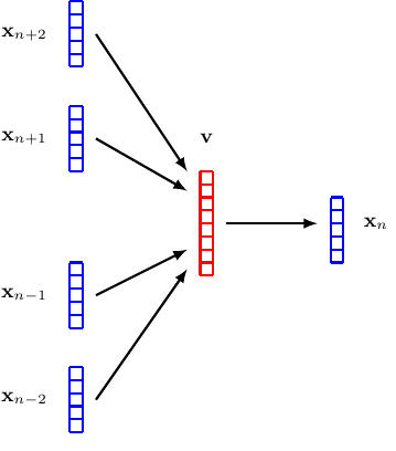
Each token id → a learned embedding vector. Training places semantically related tokens near each other.

  • a lookup table \(\mathbf{E}\in\R^{V\times D}\) (\(V\) = vocab, \(D\) = model dim)
  • learned jointly with the rest of the network (L7 backprop)
  • the geometry is the meaning (L11 representation)

Source: Bishop & Bishop (2024), Fig 12.11 — learning word embeddings from context.

Two objectives: GPT vs BERT

GPT — causal LM (decoder)

  • predict the next token, left-to-right
  • causal mask: can’t see the future
  • great at generation

BERT — masked LM (encoder)

  • randomly mask ~15% of tokens, predict them
  • bidirectional: sees both sides
  • great at understanding (classify, QA)

Same transformer, different self-supervised game → different strengths. GPT writes; BERT reads.

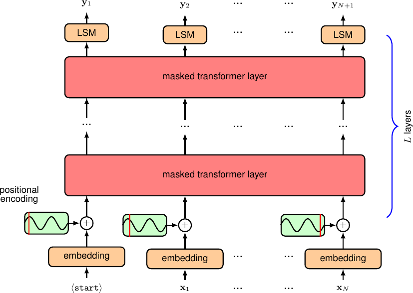
GPT: generate left-to-right

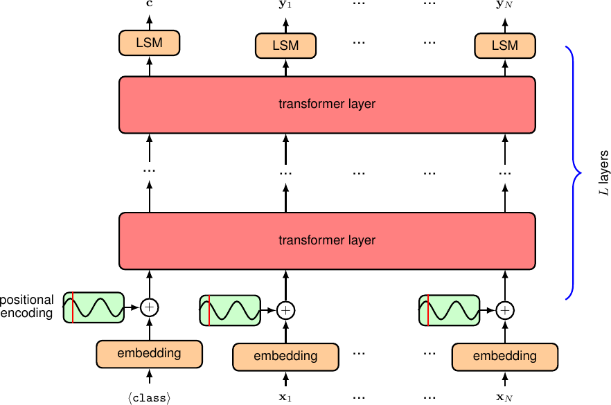
  • embed tokens + positions → stacked masked transformer layers → softmax over vocab
  • sample a token, append, repeat (autoregressive)
  • the only task is next-token prediction — yet it learns grammar, facts, reasoning

Source: Bishop & Bishop (2024), Fig 12.15 — GPT decoder.

BERT: understand both directions

  • no causal mask → every token sees all others
  • pretrain by filling masked blanks, then fine-tune a small head for the task
  • “The [MASK] sat on the mat”cat

Source: Bishop & Bishop (2024), Fig 12.18 — encoder (BERT) with a \(\langle\)class\(\rangle\) output.

Decoding: choosing the next token

The model gives a distribution; we must pick. (Bishop §12.3.2)

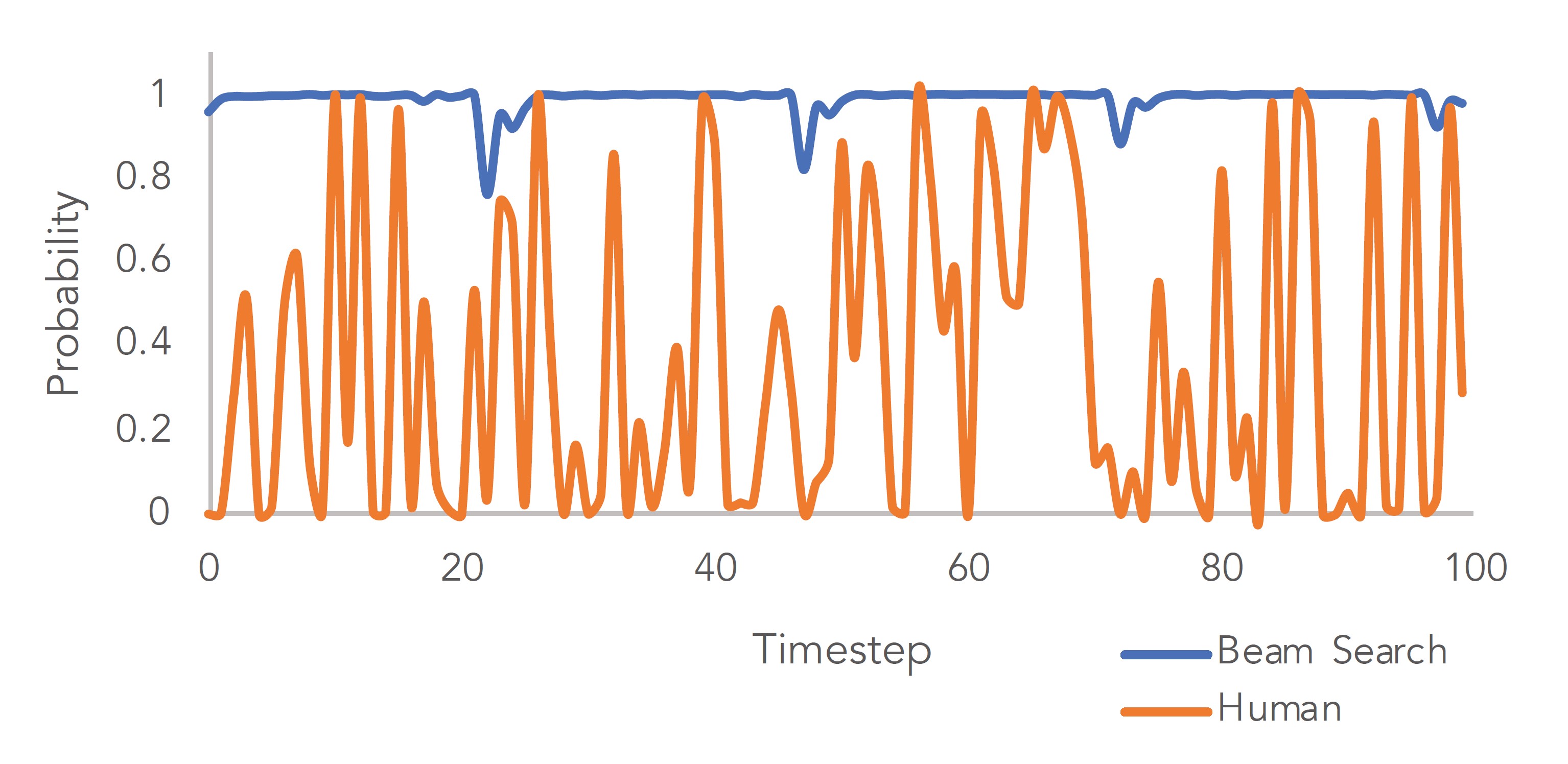
  • greedy — take the argmax → deterministic, repetitive
  • beam search — keep \(B\) best sequences → high-prob but bland
  • sampling — draw from the distribution → diverse, natural

Source: Bishop & Bishop (2024), Fig 12.17 — beam search (flat, high-prob) vs human text (varied).

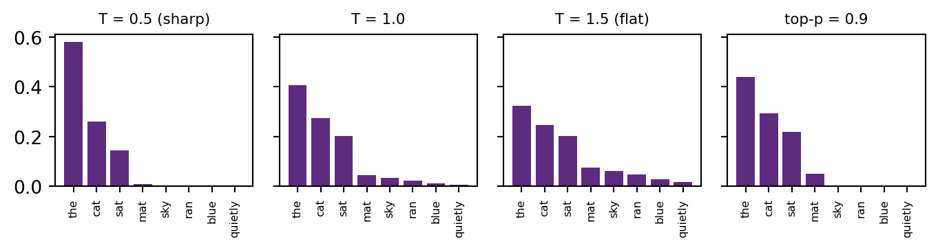
Demo: temperature, top-k, top-p

import numpy as np, matplotlib.pyplot as plt
vocab  = ["the","cat","sat","mat","sky","ran","blue","quietly"]
logits = np.array([3.2, 2.8, 2.5, 1.0, 0.7, 0.3, -0.5, -1.2])
def softmax(z): e = np.exp(z - z.max()); return e / e.sum()
def topp(p, thr):
    o = np.argsort(p)[::-1]; cum = np.cumsum(p[o]); keep = o[:np.searchsorted(cum, thr)+1]
    q = np.zeros_like(p); q[keep] = p[keep]; return q / q.sum()

dists = {"T = 0.5 (sharp)": softmax(logits/0.5), "T = 1.0": softmax(logits),
         "T = 1.5 (flat)": softmax(logits/1.5), "top-p = 0.9": topp(softmax(logits), 0.9)}
fig, ax = plt.subplots(1, 4, figsize=(7.2, 2.0), sharey=True)
for a, (t, p) in zip(ax, dists.items()):
    a.bar(range(len(vocab)), p, color="#5d2c80"); a.set_title(t, fontsize=8)
    a.set_xticks(range(len(vocab))); a.set_xticklabels(vocab, rotation=90, fontsize=6)
plt.tight_layout(); plt.show()
🔢 Measuring an LM: perplexity

Training maximizes likelihood = minimizes cross-entropy per token (L2). The standard report is its exponential, perplexity:

\[\text{PPL} = \exp\!\Big(-\tfrac1N\sum_{n} \ln p(y_n\given y_{<n})\Big)\]

Worked example: the model gave the true tokens probabilities \([0.5,\,0.25,\,0.1,\,0.4]\). \[-\tfrac14(\ln 0.5+\ln 0.25+\ln 0.1+\ln 0.4)=1.32\] \[\text{PPL}=e^{1.32}\approx 3.8\]

PPL = the effective number of equally-likely choices per step. Perfect model → 1; uniform over vocab \(V\)\(V\). Lower is better.

From pretraining to many tasks

  1. Pretrain on huge unlabelled text (self-supervised, L11)
  2. Fine-tune on a small labelled set, or…
  3. In-context learning — give examples in the prompt, no weight updates (GPT-3, Brown 2020)

Pillar: in-context / few-shot learning is emergent — small models can’t do it. It appears only at scale (L14).

Summary

  1. A language model = autoregressive \(p(y_n\mid y_{<n})\) over tokens (Bishop 12.34)
  2. Tokenization (subword) + learned embeddings turn text into vectors
  3. GPT (causal, generate) vs BERT (masked, understand) — same transformer, different objective
  4. Decoding: greedy/beam are high-prob but bland; temperature & top-k/top-p give natural text
  5. Pretrain → fine-tune → in-context — and in-context learning is emergent (L14)

Something to think about: why can’t BERT generate text autoregressively the way GPT does? (Hint: what does bidirectional attention let it “see” during training?)

📌 Read before next class

Scaling & Modern AI Systems

Scaling laws, compute-optimal training (Chinchilla), and emergent abilities — the quantitative story of “bigger is better.”

Reading: Kaplan et al., Scaling Laws for Neural Language Models (2020); Hoffmann et al., Chinchilla (2022). References: Radford et al., GPT-2 (2019); Brown et al., GPT-3 (2020); Devlin et al., BERT (2019); Holtzman et al., top-p sampling (2020). Figures from Bishop & Bishop (2024), Ch 12 — https://www.bishopbook.com/

⌂ Home