Lecture 7 — Backpropagation

Deep Learning · Session 7

Kasemsit Teeyapan

Department of Computer Engineering, Chiang Mai University

Today

The problem: get \(\nabla E\) for millions of weights — efficiently
The chain rule run backwards: error signals \(\delta\)
The two-pass algorithm (forward, then backward) — cost \(O(W)\)
Backprop = reverse-mode automatic differentiation (loss.backward())
Vanishing / exploding gradients — why depth is hard to train

Reference: Bishop & Bishop (2024), Chapter 8 — Backpropagation

Recap → the problem

You need \(\partial E/\partial w\) for a million weights. The obvious way: nudge one weight, re-run the whole net, see how \(E\) changed. How many full passes is that — and could a smarter method get all million gradients for the price of roughly one pass?

L6: train by \(\vw \leftarrow \vw - \eta\,\nabla E\)

So we need \(\dfrac{\partial E}{\partial w_{ji}}\) for every weight — and there are millions.

The naive fix (numerical): \[ \frac{\partial E}{\partial w} \approx \frac{E(w+\epsilon)-E(w)}{\epsilon} \]

one extra forward pass per weight
\(W\) weights → \(O(W^2)\) — hopeless

Backprop computes all \(W\) derivatives in a single backward pass — total cost \(O(W)\), like one extra forward pass

predict (30 วิ): ให้เดาก่อน — naive = กี่ pass? ทำดีกว่านั้นได้ไหม? อย่าเพิ่งเฉลย เชื่อม L6: ต้องการ ∂E/∂w ของทุกน้ำหนัก (เป็นล้าน) วิธีตรงไปตรงมา (numerical): รบกวนทีละน้ำหนักแล้ววัด → 1 forward pass ต่อ 1 น้ำหนัก → O(W²) ใช้ไม่ได้จริง ย้ำ pillar: backprop หา gradient ครบทุกตัวใน backward pass เดียว = O(W) (ราว ๆ forward pass เพิ่มอีกรอบ) นี่คือเหตุผลที่ deep learning เป็นไปได้จริง ~2 นาที

Why not numerical differentiation?

too slow: \(O(W^2)\) for a full gradient
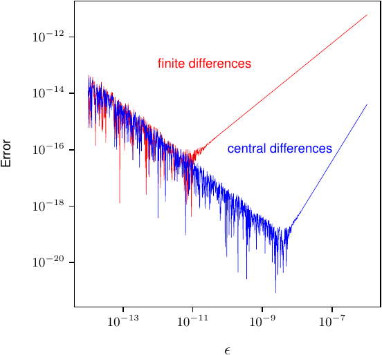
and inaccurate: large \(\epsilon\) → truncation error; tiny \(\epsilon\) → round-off blows up
(still useful for one thing: checking backprop is correct — see the demo)

Source: Bishop & Bishop (2024), Deep Learning, Fig 8.2 — error vs step size \(\epsilon\)

Part 1 · The Chain Rule on a Network

Forward, then error signals

Forward (Lecture 5): each unit computes \[ a_j = \textstyle\sum_i w_{ji}\,z_i, \qquad z_j = h(a_j) \]

Define the error signal \(\;\delta_j \equiv \dfrac{\partial E}{\partial a_j}\;\) — “how much the loss cares about unit \(j\)’s input.”

By the chain rule, the weight gradient is then simply: \[ \boxed{\;\frac{\partial E}{\partial w_{ji}} = \delta_j\, z_i\;} \qquad (\text{error} \times \text{input}) \]

Errors flow backward

Output layer (with matching loss, from L3): \[ \delta_k = y_k - t_k \]

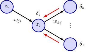
Hidden layer — collect \(\delta\) from the units it feeds: \[ \delta_j = h'(a_j)\sum_k w_{kj}\,\delta_k \]

The same weights \(w_{kj}\) used forward are reused backward — errors propagate from output to input

Source: Bishop & Bishop (2024), Deep Learning, Fig 8.1 — \(\delta_j\) from the \(\delta_k\) it connects to

The two-pass algorithm

1 · Forward pass

feed \(\vx\) through the net
compute & store all \(a_j, z_j\)

2 · Backward pass

\(\delta\) at output \(= y - t\)
propagate \(\delta_j = h'(a_j)\sum_k w_{kj}\delta_k\)
read off \(\partial E/\partial w_{ji} = \delta_j z_i\)

Two sweeps through the network — total cost \(\approx\) 2× a forward pass, independent of the number of weights per unit.

🔢 Worked example: backprop by hand

Tiny net: \(\vx\!\to\!2\) ReLU units \(\to\!1\) linear output, squared loss, target \(t=1\). Weights \(W^{(1)}=\begin{bmatrix}0.5&-0.5\\1&0.5\end{bmatrix}\), \(W^{(2)}=[\,1,\,-1\,]\), input \(\vx=[1,2]\).

Forward \[\va^{(1)}=W^{(1)}\vx=[-0.5,\;2]\] \[\vz^{(1)}=\text{ReLU}(\va^{(1)})=[0,\;2]\] \[y=W^{(2)}\vz^{(1)}=0-2=-2\] \[E=\tfrac12(y-t)^2=\tfrac12(-3)^2=4.5\]

Backward (\(\text{ReLU}'(a)=\mathbb{1}[a>0]\)) \[\delta_{\text{out}}=y-t=-3\] \[\frac{\partial E}{\partial W^{(2)}}=\delta_{\text{out}}\vz^{(1)}=[0,\;-6]\] \[\boldsymbol\delta^{(1)}=\text{ReLU}'(\va^{(1)})\odot(W^{(2)\top}\delta_{\text{out}})=[0,\;3]\] \[\frac{\partial E}{\partial W^{(1)}}=\boldsymbol\delta^{(1)}\vx^\top=\begin{bmatrix}0&0\\3&6\end{bmatrix}\]

Note unit 1’s gradient is 0 — its ReLU was off (\(a=-0.5\)), so no error flows through it. Everything is (error signal) × (input).

worked example ทำมือ (สำคัญสำหรับสอบเขียน) — เลือก ReLU เพราะ derivative เป็น 0/1 ทำให้ตัวเลขลงตัวหมด เดินให้ดูทีละขั้น: forward คำนวณ a1=[-0.5,2], ReLU→z1=[0,2], y=-2, E=4.5; backward: δ_out=y-t=-3, ∂E/∂W2=δ_out·z1=[0,-6], δ1=ReLU’(a1)⊙(W2ᵀδ_out)=[0,1]⊙[-3,3]=[0,3], ∂E/∂W1=δ1·xᵀ=[[0,0],[3,6]] จุดสอน: unit 1 มี gradient=0 เพราะ ReLU มันปิด (a=-0.5<0) → error ไม่ไหลผ่าน (dead ReLU เชื่อม vanishing gradient สไลด์ท้าย) ย้ำทุกพจน์เป็น (error signal)×(input) ให้ นศ ลองทำเองด้วยตัวเลขใหม่ ~3 นาที

✍️ Your turn: backprop by hand

Same net: \(\vx\!\to\!2\) ReLU units \(\to\!1\) linear output, squared loss. Now \(W^{(1)}=\begin{bmatrix}1&-1\\1&-3\end{bmatrix}\), \(W^{(2)}=[\,2,\,1\,]\), input \(\vx=[2,1]\), target \(t=0\).

Forward — find \(\va^{(1)}\), \(\vz^{(1)}=\text{ReLU}(\va^{(1)})\), \(y\), \(E=\tfrac12(y-t)^2\).

Backward — find \(\delta_{\text{out}}\), \(\dfrac{\partial E}{\partial W^{(2)}}\), \(\boldsymbol\delta^{(1)}\), \(\dfrac{\partial E}{\partial W^{(1)}}\).

Which hidden unit is dead here, and what is its row of \(\partial E/\partial W^{(1)}\)?

🔬 Demo: backprop vs numerical gradient

import numpy as np
rng = np.random.default_rng(0)
x = rng.standard_normal(3); t = np.array([0.5])
W1 = rng.standard_normal((4, 3)); W2 = rng.standard_normal((1, 4))

def forward(W1, W2):
    a1 = W1 @ x; z1 = np.tanh(a1); y = W2 @ z1
    return 0.5*np.sum((y - t)**2), (z1, y)

E, (z1, y) = forward(W1, W2)
dy  = y - t                       # δ at output
dW2 = np.outer(dy, z1)            # ∂E/∂W2 = δ · zᵀ
da1 = (1 - z1**2) * (W2.T @ dy)   # δ hidden = h'(a)·Wᵀδ ,  tanh'(a)=1−z²
dW1 = np.outer(da1, x)           # ∂E/∂W1 = δ · xᵀ

def numgrad(W, sel):              # finite-difference check
    g = np.zeros_like(W)
    for i in np.ndindex(W.shape):
        Wp = W.copy(); Wp[i] += 1e-6
        g[i] = (forward(*((Wp, W2) if sel == 1 else (W1, Wp)))[0] - E)/1e-6
    return g
print("max |backprop − numerical|:  W1 =", f"{abs(dW1-numgrad(W1,1)).max():.1e}",
      " W2 =", f"{abs(dW2-numgrad(W2,2)).max():.1e}")

max |backprop − numerical|:  W1 = 1.0e-07  W2 = 3.1e-07

The hand-derived backprop matches numerical gradients to \(\sim 10^{-6}\) — this gradient check is how you debug a custom layer.

Part 2 · It’s Automatic Differentiation

Backprop = reverse-mode autodiff

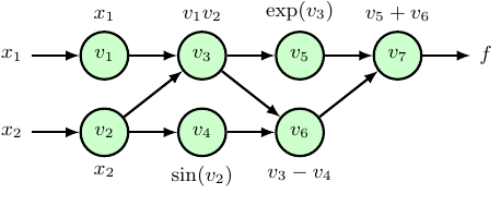
Any computation is a graph of simple ops. Autodiff applies the chain rule mechanically:

forward mode: sweep inputs → output
reverse mode: one forward (store values) + one backward (accumulate \(\partial f/\partial\,\cdot\))

Reverse mode is efficient when #outputs ≪ #inputs — a scalar loss, millions of weights = exactly our case. Backprop is reverse-mode autodiff.

Source: Bishop & Bishop (2024), Deep Learning, Fig 8.4 — an evaluation (computational) graph

Part 3 · Why Depth Is Hard to Train

Vanishing & exploding gradients

Backprop multiplies many factors: \(\;\delta_j = h'(a_j)\sum_k w_{kj}\delta_k\;\) — across \(L\) layers,

\[ \delta_{\text{early}} \sim \Big(\prod_{\ell} h'(a^{(\ell)})\,\mathbf W^{(\ell)}\Big)\,\delta_{\text{late}} \]

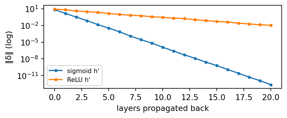
For a sigmoid, \(h'(a)\le\tfrac14\). As \(\delta\) propagates back through 20 layers, does \(\|\delta\|\) grow, stay steady, or shrink — and roughly how fast? What changes if we swap in ReLU (\(h'=1\))?

Saturating activations (sigmoid, \(h'\le\tfrac14\)) make \(\delta\) vanish exponentially → early layers barely learn. ReLU (\(h'=1\)) keeps it alive.

predict (30 วิ): ให้เดา sigmoid 20 ชั้น ‖δ‖ โต/นิ่ง/หด? เร็วแค่ไหน? ReLU ต่างไหม? อย่าเพิ่งเฉลย — รันให้ดู backprop คูณหลายปัจจัย: δ ชั้นต้น ~ ผลคูณของ h’ และ W ข้ามทุกชั้น รันสด (semilog): sigmoid h’≤¼ → ‖δ‖ หดแบบ exponential เมื่อย้อนหลายชั้น (vanishing) → ชั้นต้นแทบไม่เรียน; ReLU h’=1 → ‖δ‖ ค่อนข้างคงที่ เชื่อม L5 (ทำไม ReLU) ย้ำ pillar: นี่คือเหตุผลที่ deep ฝึกยากในอดีต ทางแก้สมัยใหม่: ReLU, careful init, normalization, residual connections (จะเจอตอน CNN/regularization) ~3 นาที

Summary

GD needs \(\partial E/\partial w_{ji}\) for every weight — numerical diff is \(O(W^2)\); backprop is \(O(W)\)
Forward stores activations; backward propagates \(\delta_j=h'(a_j)\sum_k w_{kj}\delta_k\); gradient \(=\delta_j z_i\)
It is reverse-mode autodiff — efficient because the loss is scalar (loss.backward())
Long products of \(h'\) and \(\mathbf W\) cause vanishing/exploding gradients → ReLU, init, normalization help

Something to think about: for a sigmoid, \(h'(a)=z(1-z)\le\tfrac14\). Through 10 layers, by what factor can \(\|\delta\|\) shrink in the best case? (Hint: \((\tfrac14)^{10}\).)

📌 Read before next class

Bishop & Bishop (2024), Chapter 9 — Regularization

Now we can train deep nets — how do we stop them from overfitting? Weight decay, dropout, early stopping, batch/layer normalization.

Figures from Bishop & Bishop, Deep Learning: Foundations and Concepts (2024), Chapter 8 — https://www.bishopbook.com/