\( \newcommand{\vw}{\mathbf{w}} \newcommand{\vx}{\mathbf{x}} \newcommand{\vt}{\mathbf{t}} \newcommand{\vy}{\mathbf{y}} \newcommand{\vz}{\mathbf{z}} \newcommand{\vq}{\mathbf{q}} \newcommand{\vk}{\mathbf{k}} \newcommand{\vv}{\mathbf{v}} \newcommand{\vc}{\mathbf{c}} \newcommand{\vp}{\mathbf{p}} \newcommand{\vh}{\mathbf{h}} \newcommand{\vmu}{\boldsymbol{\mu}} \newcommand{\vsigma}{\boldsymbol{\sigma}} \newcommand{\vepsilon}{\boldsymbol{\epsilon}} \newcommand{\R}{\mathbb{R}} \newcommand{\E}{\mathbb{E}} \newcommand{\norm}[1]{\lVert #1 \rVert} \newcommand{\given}{\,\vert\,} \)

Lecture 18 — Computer Vision Tasks

Deep Learning · Detection & Segmentation

Kasemsit Teeyapan

Department of Computer Engineering, Chiang Mai University

Today

  1. Beyond classification: the vision task spectrumwhat, where, which pixels
  2. Object detection = classify + localize (a multi-task problem, L17)
  3. IoU and non-max suppression — measuring and cleaning up boxes
  4. Detection architectures: R-CNN family, one-stage (YOLO), DETR
  5. Semantic segmentation and the U-Net encoder–decoder

Reference: Bishop & Bishop (2024), §10.4 (object detection) & §10.5 (image segmentation)

Recap → the vision task spectrum

  • classification (L9): one label per image — “a cat”
  • detection: a box + class for each object — “cat here, dog there”
  • semantic segmentation: a class for every pixel
  • instance segmentation: pixels + which object

Each step asks for more spatial detail. The CNN features from L9 stay the backbone — we just change the head and the loss.

Object detection = classify + localize

For each object, output two things:

  • class — a softmax (L3) over categories
  • box — 4 numbers \((x, y, w, h)\) via regression (L2)

\[\mathcal L = \mathcal L_{\text{cls}} + \lambda\,\mathcal L_{\text{box}}\]

Pillar: detection is multi-task learning (L17) — one shared backbone, a classification head and a box-regression head, trained with a combined loss.

Measuring a box: IoU

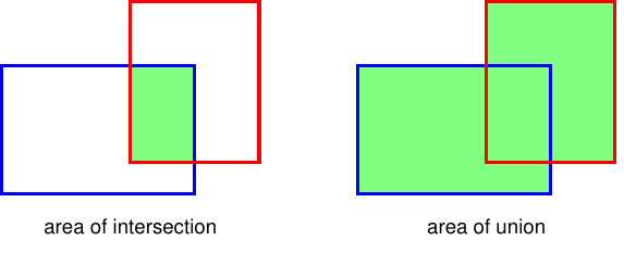
Intersection-over-Union — overlap of predicted vs ground-truth box:

\[\text{IoU} = \frac{\text{area of intersection}}{\text{area of union}} \in [0,1]\]

  • a prediction is “correct” if \(\text{IoU} > 0.5\) (typical)
  • not used as a loss directly — hard to optimize by gradient descent

Source: Bishop & Bishop (2024), Fig 10.20 — intersection (left) over union (right).

Too many boxes: NMS

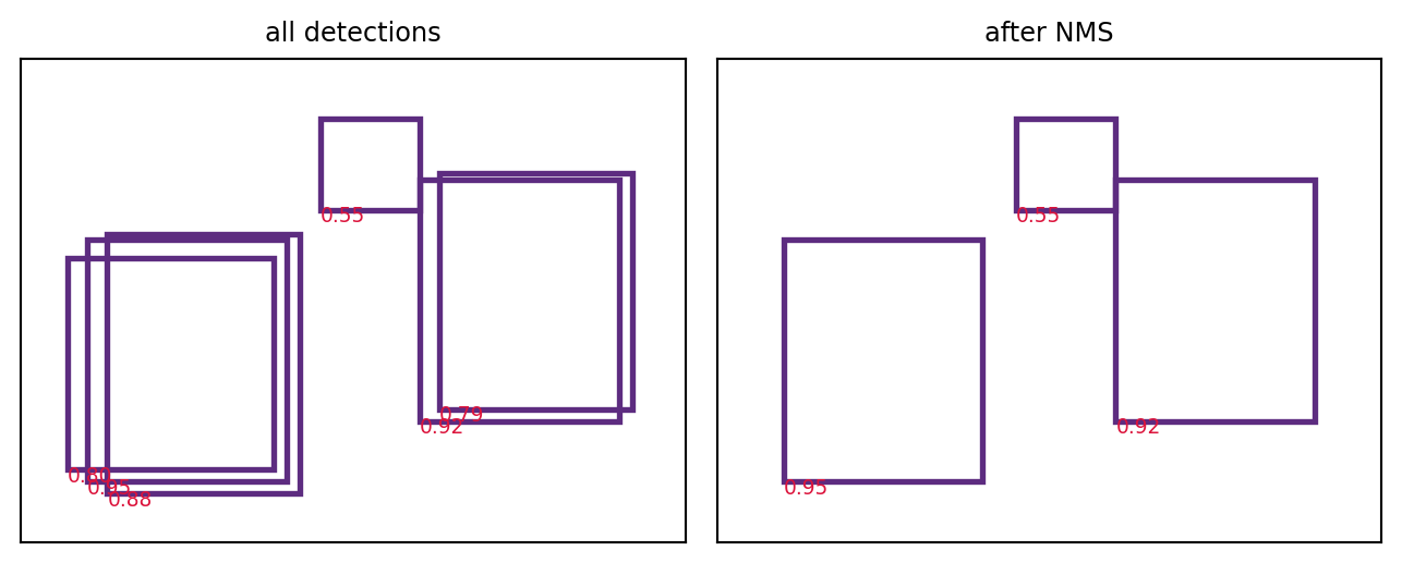
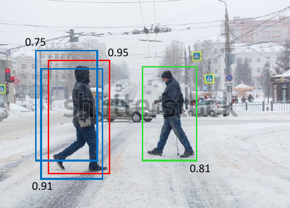
Scanning detectors fire many overlapping boxes on one object. Non-max suppression cleans up, per class:

  1. take the highest-confidence box → keep it
  2. discard boxes with IoU > 0.5 against it
  3. repeat on the rest

→ one box per object, other instances preserved.

Source: Bishop & Bishop (2024), Fig 10.25 — keep the max (red/green), suppress overlaps (blue).

Demo: IoU + non-max suppression

import numpy as np, matplotlib.pyplot as plt
from matplotlib.patches import Rectangle
boxes = np.array([[1,1,4,5],[1.3,0.8,4.2,5.1],[0.7,1.2,3.8,4.7],
                  [6,2,9,6],[6.3,2.2,9.2,6.1],[4.5,5.5,6,7]], float)
scores = np.array([0.95,0.88,0.80, 0.92,0.79, 0.55])
def iou(a,b):
    x1,y1=max(a[0],b[0]),max(a[1],b[1]); x2,y2=min(a[2],b[2]),min(a[3],b[3])
    inter=max(0,x2-x1)*max(0,y2-y1)
    return inter/((a[2]-a[0])*(a[3]-a[1])+(b[2]-b[0])*(b[3]-b[1])-inter)
def nms(b,s,thr=0.5):
    idx=list(np.argsort(s)[::-1]); keep=[]
    while idx:
        i=idx.pop(0); keep.append(i); idx=[j for j in idx if iou(b[i],b[j])<thr]
    return keep
keep=nms(boxes,scores)
fig,ax=plt.subplots(1,2,figsize=(6.8,2.8))
for a,sel,t in [(ax[0],range(len(boxes)),"all detections"),(ax[1],keep,"after NMS")]:
    for k in sel:
        x1,y1,x2,y2=boxes[k]
        a.add_patch(Rectangle((x1,y1),x2-x1,y2-y1,fill=False,ec="#5d2c80",lw=2))
        a.text(x1,y1-.2,f"{scores[k]:.2f}",fontsize=7,color="crimson")
    a.set_xlim(0,10); a.set_ylim(0,8); a.set_title(t,fontsize=9); a.set_xticks([]); a.set_yticks([])
plt.tight_layout(); plt.show()
Detection architectures

Two-stage (propose, then classify)

  • R-CNN → Fast → Faster R-CNN: a region-proposal network finds candidates, a head classifies + refines boxes
  • accurate, slower

One-stage / end-to-end

  • YOLO / SSD: predict all boxes in one pass → real-time
  • DETR: a transformer (L10) predicts a set of boxes directly — no NMS, no anchors

The trend: fewer hand-designed steps (proposals, anchors, NMS) → more learned end-to-end (the Bitter Lesson, L14).

Semantic segmentation

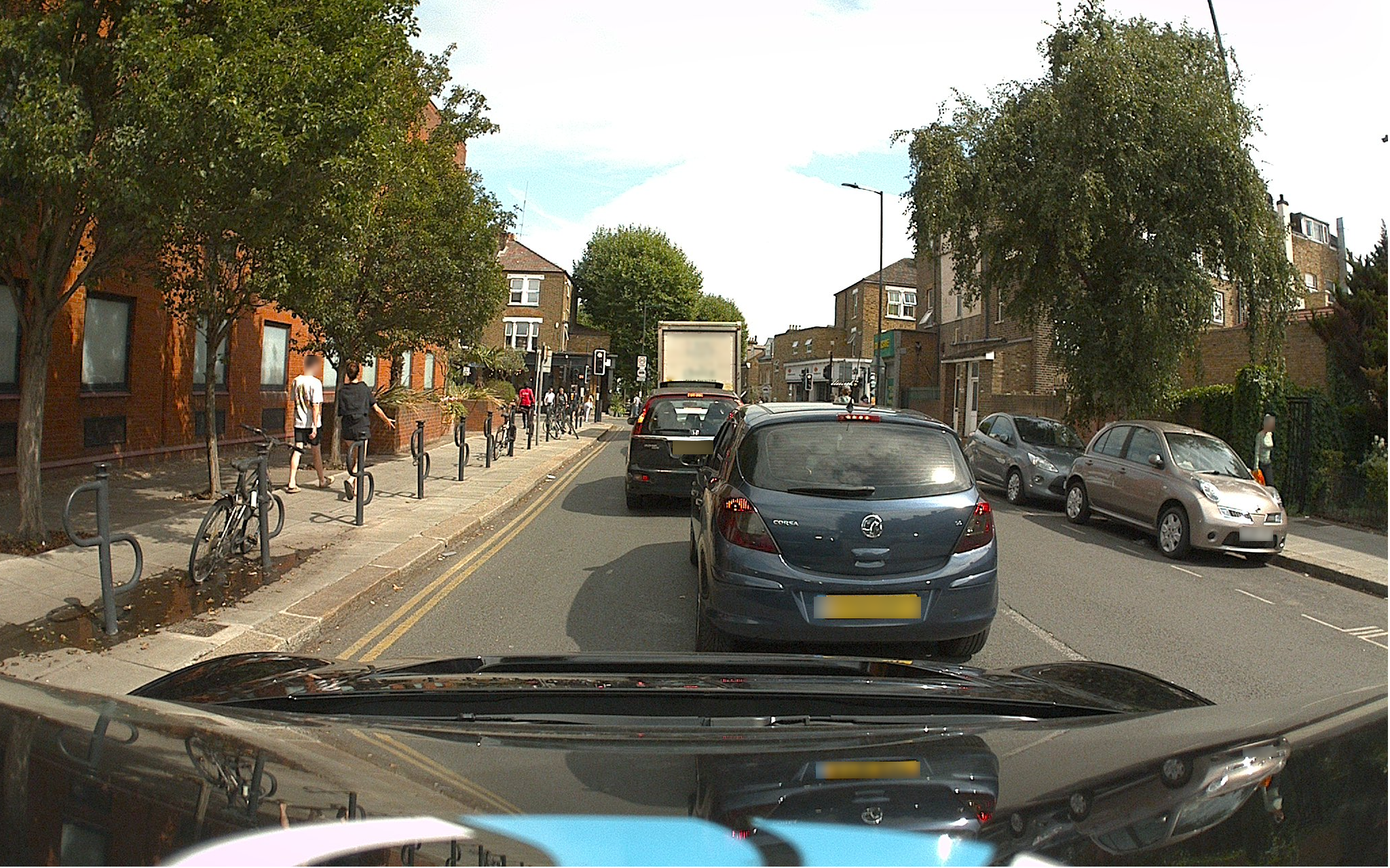
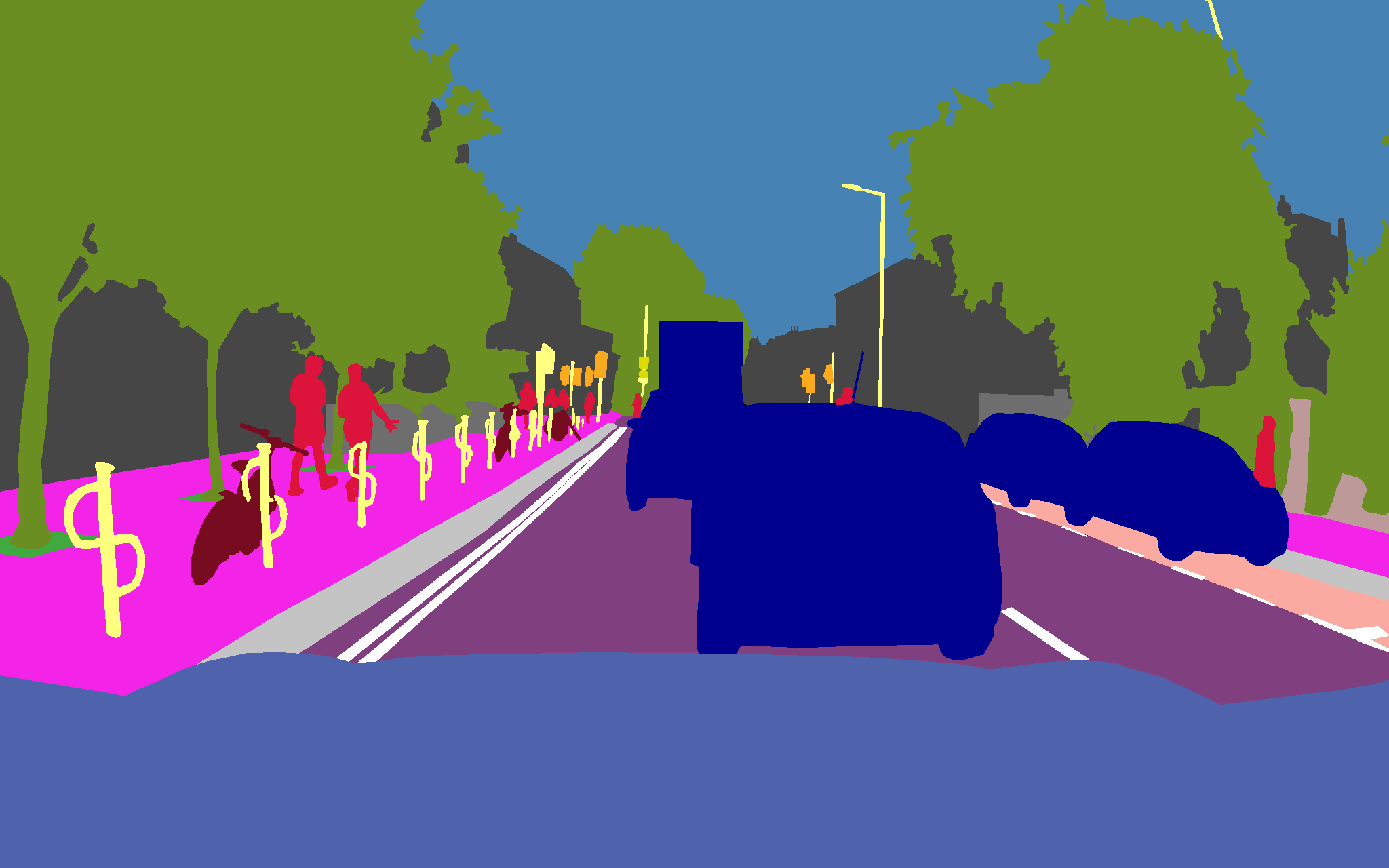
Classify every pixel → output has the same \(H\times W\) as the input, with \(C\) class channels.

  • it’s dense classification: a softmax (L3) per pixel
  • needs both global context (what) and fine spatial detail (where)

Source: Bishop & Bishop (2024), Fig 10.26 — an image and its semantic segmentation.

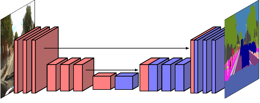
The U-Net: encoder–decoder + skips

  • encoder downsamples → captures context (what), loses resolution
  • decoder upsamples → restores resolution (where)
  • skip connections copy fine detail across (L8!) so edges stay sharp
  • upsampling via transposed conv / unpooling

Source: Bishop & Bishop (2024), Fig 10.31 — the U-Net (down-sampling ↔︎ up-sampling, with skips).

Pillar: the same skip-connection idea that saved gradients in deep nets (L8) here carries spatial detail past the bottleneck.

Putting it together

  • semantic: every pixel a class (road, sky, car)
  • instance: separate each object (car #1 vs car #2)
  • panoptic: both at once
  • Mask R-CNN: Faster R-CNN + a mask head → detection and per-object masks

Modern frontier: ViT backbones (L10) and promptable models like SAM (Segment Anything) — segment objects from a click or text, zero-shot.

Summary

  1. Vision task spectrum: classification → detection → segmentation (more spatial detail each step)
  2. Detection = multi-task (L17): shared backbone + class head + box-regression head
  3. IoU measures box overlap; NMS removes duplicate boxes (a few lines of code)
  4. Architectures: R-CNN familyYOLODETR (fewer hand-designed steps, L14)
  5. Segmentation = per-pixel classification; U-Net = encoder–decoder with skips (L8)

Something to think about: DETR predicts a fixed set of boxes with a transformer and needs no NMS. What must its training loss do to make duplicate predictions unnecessary? (Hint: it matches predictions to ground-truth as a set.)

📌 Closing

The CNN backbone (L9) + transformers (L10) + multi-task heads (L17) compose into detection and segmentation — the workhorses of real-world vision.

Same primitives, new task. That is the whole game.

References: Girshick, Fast R-CNN (2015); Ren et al., Faster R-CNN (2015); Redmon et al., YOLO (2016); Carion et al., DETR (2020); Ronneberger et al., U-Net (2015); He et al., Mask R-CNN (2017); Kirillov et al., Segment Anything (2023). Figures from Bishop & Bishop (2024), Ch 10 — https://www.bishopbook.com/

⌂ Home