Lecture 3 — Single-layer Networks: Classification

Deep Learning · Session 3

Kasemsit Teeyapan

Department of Computer Engineering, Chiang Mai University

Today

From predicting numbers to predicting classes
Why plain least squares fails for classification
Logistic regression: the sigmoid, and cross-entropy from maximum likelihood
Multi-class: softmax & categorical cross-entropy
Decision theory: from probabilities to optimal actions (costs, the reject option)
Nonlinear classification via basis functions → a bridge to deep nets

Reference: Bishop & Bishop (2024), Chapter 5 — Single-layer Networks: Classification

Recap → today

Lecture 2 (regression):

model \(y=\vw^{\mathsf T}\boldsymbol{\phi}(\vx)\)
Gaussian noise → squared-error loss
= maximum likelihood

Today (classification):

output a probability of each class
Bernoulli / Categorical → cross-entropy loss
= maximum likelihood (same recipe!)

Same recipe, different noise model: choose a distribution for the target → the negative log-likelihood is your loss

Part 1 · From Regression to Classification

The task & a linear decision boundary

Targets are now discrete classes. For \(K\) classes use 1-of-K (one-hot): class 2 of 3 → \(\vt=(0,1,0)\).

A linear model splits input space with a decision boundary:

\[ a(\vx) = \vw^{\mathsf T}\vx + b \]

\(a(\vx) > 0\) → class 1, else class 2
boundary is where \(a(\vx)=0\) (a line / hyperplane)

\(\vw\) is perpendicular to the boundary
direction of \(\vw\) = “which way is class 1”

But a raw score \(a(\vx)\) is not a probability — we will fix that.

Could we just use least squares?

Labels are \(t\in\{0,1\}\). We could fit them with the regression line from Lecture 2.

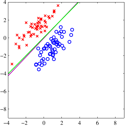
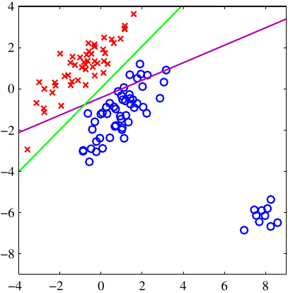
Add a cluster of points that are clearly class 1 but far from the boundary. Will the least-squares boundary stay put (those points are already correct) or swing toward them? Watch the next slide.

Why not least squares?

Add a few far-away points (right) and the least-squares boundary (magenta) swings away and misclassifies — while logistic regression (green) stays sensible.

Least squares penalizes being “too correct” — wrong noise model for class labels

Source: Bishop & Bishop (2024), Deep Learning, Fig 5.4

Part 2 · Logistic Regression

Squashing a score into a probability

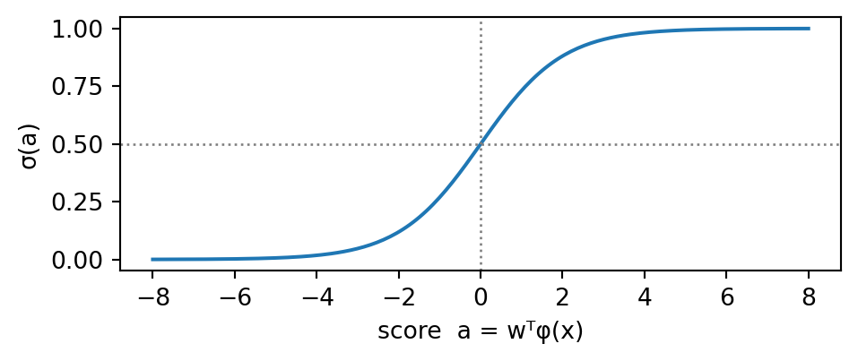
We need outputs in \([0,1]\). Pass the score through the logistic sigmoid:

\[ \sigma(a) = \frac{1}{1+e^{-a}}, \qquad p(\mathcal{C}_1\given\vx) = y(\vx) = \sigma\!\big(\vw^{\mathsf T}\boldsymbol{\phi}(\vx)\big) \]

The loss: cross-entropy from MLE

Each label is Bernoulli: \(p(t\given\vx)=y^{\,t}(1-y)^{1-t}\), with \(t\in\{0,1\}\).

Negative log-likelihood over the dataset → the cross-entropy error:

\[ E(\vw) = -\sum_{n=1}^{N}\Big\{ t_n\ln y_n + (1-t_n)\ln(1-y_n) \Big\} \]

Cross-entropy = MLE under a Bernoulli target — the mirror image of “squared error = MLE under Gaussian” (Lecture 2)

Worked example: the cost of being confident

A point gets score \(a=\vw^{\mathsf T}\boldsymbol\phi=1.0\), so the model leans class 1.

If this point’s true label is actually \(t=0\) (the model is confidently wrong), is its cross-entropy loss just a little bigger than the \(t=1\) case — or a lot?

\(y=\sigma(1)=\dfrac{1}{1+e^{-1}}=0.731\), and \(\text{loss}=-[\,t\ln y+(1-t)\ln(1-y)\,]\):

correct (\(t=1\)): \(-\ln 0.731 = \mathbf{0.31}\)
wrong (\(t=0\)): \(-\ln(1-0.731)=-\ln 0.269 = \mathbf{1.31}\)

Confident and wrong costs ~4× more — cross-entropy punishes overconfidence, exactly why it beats squared error for labels.

Your turn

A point has score \(a=2.0\).

Compute the predicted probability \(y=\sigma(2)\).
Find the cross-entropy loss if the true label is \(t=1\), and if \(t=0\).
By what factor is “confidently wrong” worse than “confidently right” here?

Training: no closed form, but a clean gradient

Unlike regression, there is no closed-form solution — minimize by gradient descent. The gradient is strikingly simple:

\[ \nabla_{\vw} E = \sum_{n=1}^{N} \big(y_n - t_n\big)\,\boldsymbol{\phi}(\vx_n) \]

Exactly the same form as linear regression — (prediction − target) × input. The sigmoid’s nonlinearity cancels neatly against the cross-entropy.

Bishop §5.4.3 — the sigmoid + cross-entropy pairing is a canonical link

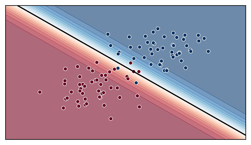
🔬 Demo: logistic regression by gradient descent

import numpy as np, matplotlib.pyplot as plt
rng = np.random.default_rng(0)
X = np.vstack([rng.normal([-1, -1], 0.8, (50, 2)),
               rng.normal([1.3, 1.3], 0.8, (50, 2))])
y = np.r_[np.zeros(50), np.ones(50)]
Xb = np.c_[np.ones(len(X)), X]; w = np.zeros(3)
for _ in range(800):                                   # gradient descent
    p = 1/(1 + np.exp(-Xb @ w))
    w -= 0.1 * Xb.T @ (p - y) / len(y)                 # ∇E = Σ (y−t) x
xx, yy = np.meshgrid(np.linspace(-4, 4, 200), np.linspace(-4, 4, 200))
P = 1/(1 + np.exp(-np.c_[np.ones(xx.size), xx.ravel(), yy.ravel()] @ w))
plt.figure(figsize=(4.6, 2.7))
plt.contourf(xx, yy, P.reshape(xx.shape), levels=20, cmap="RdBu", alpha=.6)
plt.contour(xx, yy, P.reshape(xx.shape), levels=[0.5], colors="k")
plt.scatter(X[:, 0], X[:, 1], c=y, cmap="RdBu", edgecolor="white", s=22, linewidths=0.6)
plt.xticks([]); plt.yticks([]); plt.tight_layout(); plt.show()

Part 3 · Multiple Classes: Softmax

Softmax & categorical cross-entropy

For \(K\) classes, compute a score per class \(a_k=\vw_k^{\mathsf T}\boldsymbol{\phi}(\vx)\) and normalize with softmax:

\[ y_k = p(\mathcal{C}_k\given\vx) = \frac{e^{a_k}}{\sum_{j=1}^{K} e^{a_j}} \quad\Big(y_k>0,\ \textstyle\sum_k y_k = 1\Big) \]

With one-hot targets \(t_{nk}\), the loss is categorical cross-entropy:

\[ E(\vw) = -\sum_{n=1}^{N}\sum_{k=1}^{K} t_{nk}\,\ln y_{nk} \]

\(K=2\) softmax = the sigmoid. Softmax + cross-entropy is the standard output layer of almost every classifier you will build.

Worked example: softmax on real numbers

Three class scores (logits) \(\mathbf a=(2,\,1,\,0)\).

Class 1 has the largest logit, by a gap of just 1. Guess its probability: more or less than \(\tfrac{2}{3}\)?

\(e^{2},\,e^{1},\,e^{0}=7.39,\ 2.72,\ 1.00\); sum \(=11.11\). \[\mathbf y=\Big(\tfrac{7.39}{11.11},\ \tfrac{2.72}{11.11},\ \tfrac{1.00}{11.11}\Big)=(0.665,\ 0.245,\ 0.090)\] If the true class is the 2nd: cross-entropy \(=-\ln 0.245 = \mathbf{1.41}\).

A 1-unit logit gap gives only \(0.665\) — softmax is “soft”, it keeps mass on the runners-up.

Your turn

Logits \(\mathbf a=(1,\,3,\,0)\).

Compute the softmax probabilities \(\mathbf y\).
Which class wins, and with what probability?
If the true class is the 2nd, what is the cross-entropy loss?

Part 4 · From Probabilities to Decisions

Inference vs decision

Logistic/softmax gives us \(p(\mathcal C_k\given\vx)\) — that was inference. But we must still act: treat the patient or not?

To minimize the misclassification rate, assign \(\vx\) to the class with the largest posterior:

\[\hat k = \arg\max_k\; p(\mathcal C_k \given \vx)\]

Pillar: this is the Bayes-optimal classifier — no rule beats picking the most probable class, if costs are symmetric. The decision step is trivial once inference gives us the probabilities.

Bishop & Bishop (2024), §5.2 (and §4.2 for regression) — Decision Theory

แยกสองขั้นให้ชัด (Bishop §5.2): inference = หา p(C_k|x) (สิ่งที่ logistic/softmax ทำ), decision = ตัดสินใจลงมือ (รักษาหรือไม่) ถ้าเป้าหมายคือ “ผิดน้อยที่สุด” กฎ optimal คือเลือกคลาสที่ posterior สูงสุด = Bayes classifier ไม่มีกฎไหนชนะได้ “ถ้า cost สมมาตร” ย้ำ: ขั้น decision ง่ายมาก เมื่อ inference ให้ probability มาแล้ว — ความยากทั้งหมดอยู่ที่หา p(C_k|x) สไลด์ถัดไปจะเห็นว่าพอ cost ไม่สมมาตร เรื่องเปลี่ยน ~2 นาที

When mistakes cost differently

A loss matrix \(L_{kj}\) = cost of predicting \(j\) when truth is \(k\). Minimize expected loss → assign \(\vx\) to

\[\arg\min_j \sum_k L_{kj}\,p(\mathcal C_k\given\vx)\]

Melanoma (L0): missing a cancer (FN) is far worse than a false alarm (FP). Say \(L_{\text{FN}}=100,\ L_{\text{FP}}=1\).

The default threshold is \(0.5\). With FN \(100\times\) worse than FP, does the “predict cancer” threshold move up or down — and roughly how far?

Predict cancer when its expected loss is smaller:

\[1\cdot p(\text{benign}\given\vx) < 100\cdot p(\text{cancer}\given\vx)\]

\[\Rightarrow\ p(\text{cancer}\given\vx) > \tfrac{1}{101}\approx 0.01\]

The threshold drops from 0.5 → 0.01: flag cancer even at 1% probability.

loss matrix L_kj = cost ของการทำนาย j เมื่อความจริงเป็น k เป้าหมายเปลี่ยนจาก “ผิดน้อยสุด” เป็น “expected loss น้อยสุด” → assign x ไปคลาสที่ Σ_k L_kj p(C_k|x) ต่ำสุด worked example melanoma (เชื่อม L0): พลาดมะเร็ง (FN) แพงกว่าเตือนผิด (FP) มาก ตั้ง L_FN=100, L_FP=1 ทำนาย “มะเร็ง” เมื่อ 1·p(benign) < 100·p(cancer) → p(cancer|x) > 1/101 ≈ 0.01 ผลคือ threshold เลื่อนจาก 0.5 เหลือ 0.01 — แจ้งเตือนมะเร็งแม้ความน่าจะเป็นแค่ 1%! นี่คือเหตุผลที่ระบบแพทย์จริงตั้ง threshold ต่ำ ให้ นศ เห็นว่า cost asymmetry เปลี่ยนการตัดสินใจอย่างไร (สอบเขียนชอบออก) ~2.5 นาที

The reject option

When the model is unsure, it can abstain instead of guessing:

predict only if \(\max_k p(\mathcal C_k\given\vx) > \theta\)
otherwise defer to a human

Trades coverage for accuracy on what it does answer.

This is exactly selective prediction (L15). It only works if the probabilities are calibrated — another reason inference quality matters.

Part 5 · Beyond Linear

Nonlinear classes? Use basis functions

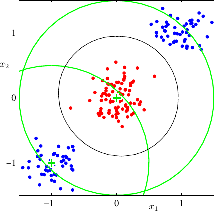
input space \(\vx\) — not separable

feature space \(\boldsymbol{\phi}(\vx)\) — linearly separable

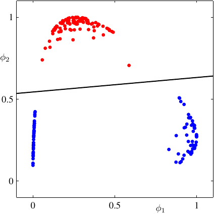
A fixed basis can make classes separable — but the next leap is to learn the features. That is the deep network.

Source: Bishop & Bishop (2024), Deep Learning, Fig 5.15 — two Gaussian basis functions map the data to a separable space

Summary

Classification predicts a probability per class, not a raw score
Logistic/softmax + cross-entropy comes from maximum likelihood (Bernoulli/Categorical) — the mirror of regression’s squared error
No closed form → gradient descent, with the clean gradient \((y-t)\,\boldsymbol{\phi}\)
Decision theory: minimize expected loss; asymmetric costs shift the threshold; abstain when unsure
Fixed basis functions handle nonlinearity — learning them is the deep network

Something to think about: show that for \(K=2\) the softmax reduces exactly to the logistic sigmoid. (Hint: divide numerator and denominator by \(e^{a_1}\).)

📌 Read before next class

Next session: Statistical Learning & Generalization — why and when models generalize.

Reading: Bishop & Bishop (2024) §4.3 (bias–variance); optional Shalev-Shwartz & Ben-David, Understanding Machine Learning (ERM, capacity, VC dimension).

Figures from Bishop & Bishop, Deep Learning: Foundations and Concepts (2024), Chapter 5 — https://www.bishopbook.com/