\( \newcommand{\vw}{\mathbf{w}} \newcommand{\vx}{\mathbf{x}} \newcommand{\vt}{\mathbf{t}} \newcommand{\vy}{\mathbf{y}} \newcommand{\vz}{\mathbf{z}} \newcommand{\vq}{\mathbf{q}} \newcommand{\vk}{\mathbf{k}} \newcommand{\vv}{\mathbf{v}} \newcommand{\vc}{\mathbf{c}} \newcommand{\vp}{\mathbf{p}} \newcommand{\vh}{\mathbf{h}} \newcommand{\vmu}{\boldsymbol{\mu}} \newcommand{\vsigma}{\boldsymbol{\sigma}} \newcommand{\vepsilon}{\boldsymbol{\epsilon}} \newcommand{\R}{\mathbb{R}} \newcommand{\E}{\mathbb{E}} \newcommand{\norm}[1]{\lVert #1 \rVert} \newcommand{\given}{\,\vert\,} \)

Lecture 11 — Representation Learning & Self-Supervised Learning

Deep Learning · Session 11

Kasemsit Teeyapan

Department of Computer Engineering, Chiang Mai University

Today

  1. Representation learning — the real goal behind every deep network
  2. Autoencoders: encode → bottleneck → reconstruct (linear AE = PCA)
  3. Self-supervised learning: free labels from the data itself (denoising, masking)
  4. Contrastive learning & SimCLR — pull positives together, push negatives apart
  5. Transfer learning — pretrain once, adapt cheaply (the foundation-model recipe)

Reference: Bishop & Bishop (2024), §6.3 (representation learning) & Chapter 19 (autoencoders)

Recap → the thread all along

  • L0: deep learning = representation learning
  • L9: CNN learns edges → parts → objects
  • L10: GPT learns from predicting the next token — no human labels

The problem: labels are expensive. The internet has near-infinite unlabelled data.

Can we learn good representations from raw, unlabelled data — then reuse them for many tasks with few labels?

What makes a representation good?

  • Distributed — many units, each a reusable factor (not one-hot) §6.3.2
  • Hierarchical — simple → complex, layer by layer §6.3.1
  • Transferable — useful for tasks it wasn’t trained on
  • Semantic — distances mean something (cat near dog, far from truck)

A representation is a learned map \(f_w:\; \vx \mapsto \vz\) into a space where downstream tasks become easy — ideally a simple (linear) classifier suffices.

Autoencoders

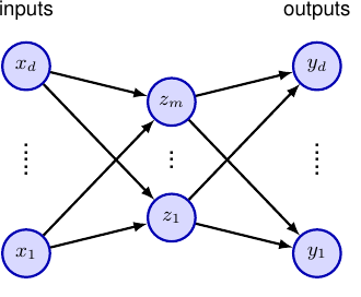
Train a network to reconstruct its own input through a bottleneck:

\[\vz = f_{\text{enc}}(\vx), \quad \hat{\vx} = f_{\text{dec}}(\vz)\] \[E(w) = \sum_n \norm{\vx_n - \hat{\vx}_n}^2\]

  • no labels — the target is the input
  • the narrow \(\vz\) forces a compressed code → keep only what matters

Source: Bishop & Bishop (2024), Fig 19.1 — an autoencoder with a bottleneck \(\vz\).

Linear autoencoder = PCA

With linear encoder/decoder and squared loss, the optimal bottleneck spans the top principal components (Bishop §19.1.1).

  • autoencoders generalize PCA to nonlinear codes
  • gives us a clean, training-free way to see representation learning

Pillar: representation learning isn’t magic — its simplest case is PCA. Depth + nonlinearity buy curved manifolds PCA can’t reach.

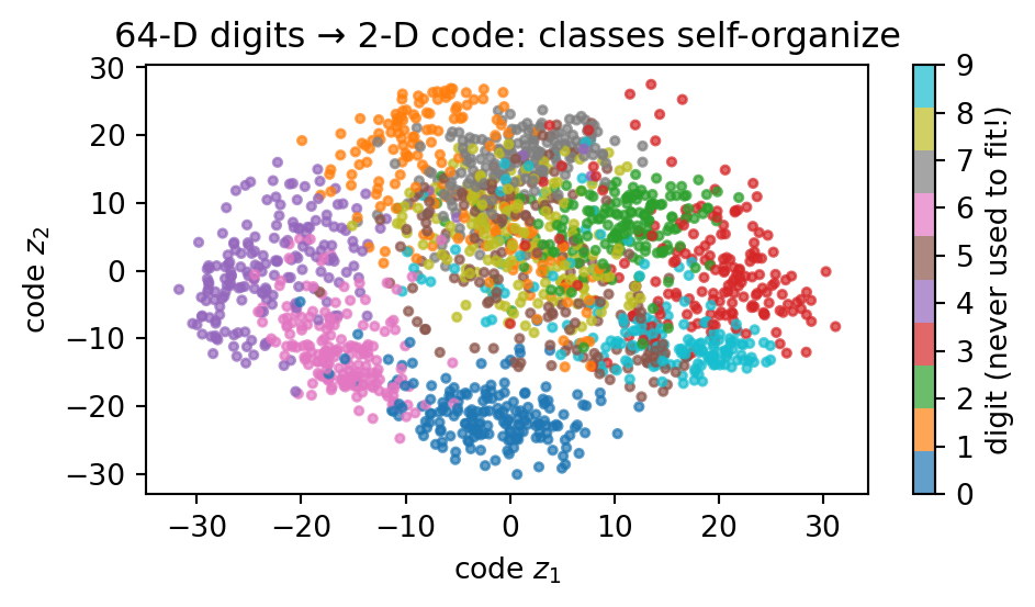
Demo: a representation emerges (PCA)

import numpy as np, matplotlib.pyplot as plt
from sklearn.datasets import load_digits

d = load_digits()
X = d.data - d.data.mean(0)                       # 1797 images, 64-D (8x8)
U, S, Vt = np.linalg.svd(X, full_matrices=False)  # linear AE optimum = PCA
Z = X @ Vt[:2].T                                  # 2-D bottleneck code

plt.figure(figsize=(5.2, 3.0))
sc = plt.scatter(Z[:, 0], Z[:, 1], c=d.target, cmap="tab10", s=8, alpha=0.7)
plt.colorbar(sc, label="digit (never used to fit!)", ticks=range(10))
plt.xlabel("code $z_1$"); plt.ylabel("code $z_2$")
plt.title("64-D digits → 2-D code: classes self-organize"); plt.tight_layout(); plt.show()
Self-supervised: free labels

Invent a pretext task whose answer is already in the data:

  • denoising AE — corrupt input, recover clean
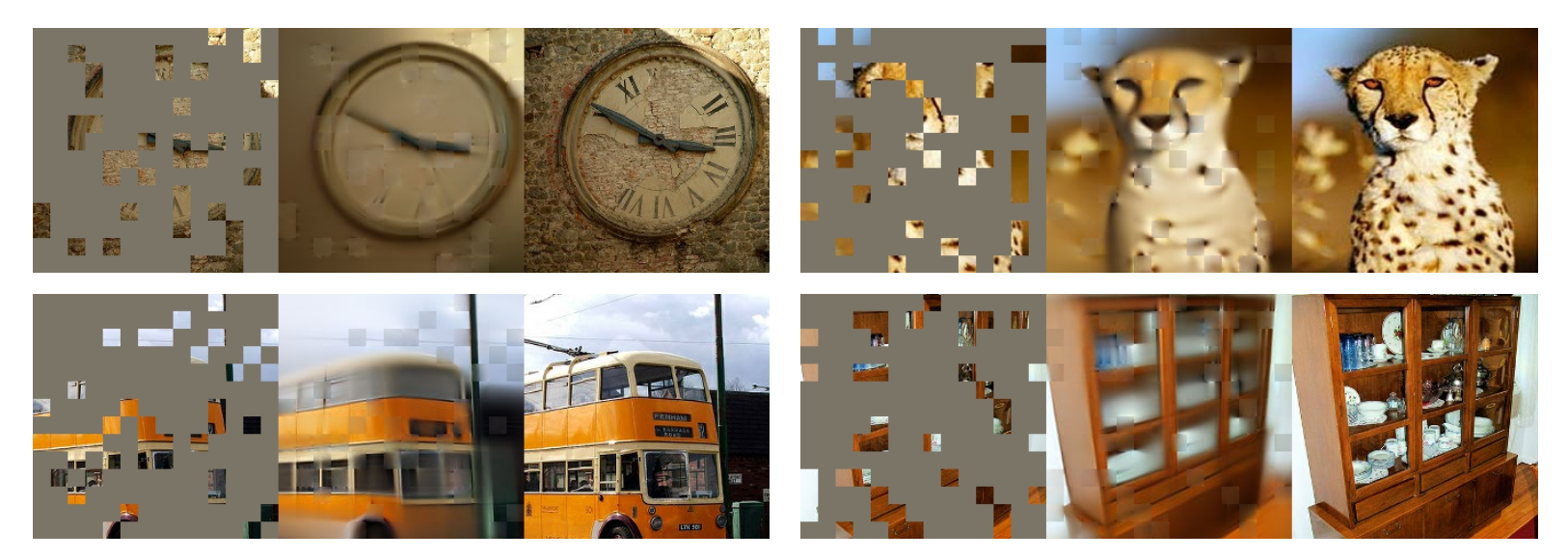
  • masked AE — hide patches, predict them (Fig 19.6)
  • next token — GPT (L10)
  • masked token — BERT (L10)

The network must understand structure to succeed.

Source: Bishop & Bishop (2024), Fig 19.6 — masked autoencoder: masked input · reconstruction · original.

Contrastive learning

Learn a space by comparison, not reconstruction:

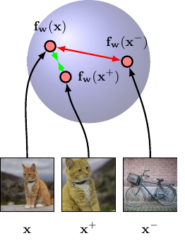
  • positive pair \((\vx, \vx^+)\) — semantically similar → pull together
  • negative pairs \((\vx, \vx^-_n)\) — dissimilar → push apart

InfoNCE loss (Bishop 6.20):

\[E = -\ln\frac{e^{\,f(\vx)^\top f(\vx^+)}}{e^{\,f(\vx)^\top f(\vx^+)} + \sum_n e^{\,f(\vx)^\top f(\vx^-_n)}}\]

Source: Bishop & Bishop (2024), Fig 6.14 — anchor \(\vx\), positive \(\vx^+\), negative \(\vx^-\) on the embedding sphere.

SimCLR: where do positive pairs come from?

Augmentation! Two random augmentations of the same image = a positive pair; all other images in the batch = negatives.

  • crop, colour-jitter, blur… (the invariances we want, L8)
  • no labels at all
  • then: freeze \(f_w\), train a linear classifier on top → near-supervised accuracy

The choice of augmentations defines what “similar” means — i.e. it encodes the inductive bias (L8/L9) by hand.

Transfer learning

Pretrain a big model on huge unlabelled data → reuse it:

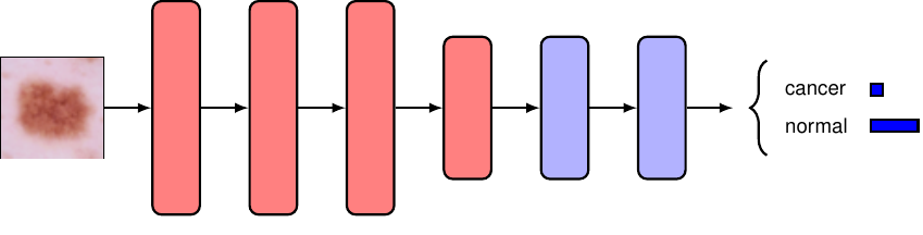
  • keep early layers (generic features)
  • swap & fine-tune the head for the new task
  • works with few labels — features already learned

Connects to L0’s melanoma classifier ↓

Source: Bishop & Bishop (2024), Fig 6.13 — transfer to a skin-cancer task; red = reused, blue = retrained.

Pillar: this is the foundation-model recipe — pretrain once at scale (L13), adapt everywhere cheaply.

Why this changed everything

  • supervised learning is bottlenecked by labels
  • self-supervised learning unlocks all the data
  • representations transfer → one pretrained model serves many tasks

GPT, BERT, CLIP, modern vision models — all are self-supervised pretraining + a little adaptation. Scale makes it work (L13).

Summary

  1. The goal of deep learning is a good representation \(f_w: \vx \mapsto \vz\)
  2. Autoencoders compress through a bottleneck; linear AE = PCA
  3. Self-supervised learning makes labels from the data (denoising, masking, next-token)
  4. Contrastive learning (InfoNCE) pulls positives together; SimCLR = augmentations as positives
  5. Transfer learning = pretrain once, adapt cheaply — the foundation-model recipe

Something to think about: in contrastive learning, what fails if your negatives are too easy (e.g. always a totally different category)? (Hint: what gradient signal do trivial negatives give?)

📌 Read before next class

Generative Models — VAEs, GANs, and Diffusion

From understanding data to generating it: learn the distribution \(p(\vx)\) and sample new examples.

Reading: Kingma & Welling, Auto-Encoding Variational Bayes (VAE) (2014). References: Chen et al., SimCLR (2020); He et al., Masked Autoencoders (2022). Figures from Bishop & Bishop (2024), §6.3 & Ch 19 — https://www.bishopbook.com/

⌂ Home