\( \newcommand{\vw}{\mathbf{w}} \newcommand{\vx}{\mathbf{x}} \newcommand{\vt}{\mathbf{t}} \newcommand{\vy}{\mathbf{y}} \newcommand{\vz}{\mathbf{z}} \newcommand{\vq}{\mathbf{q}} \newcommand{\vk}{\mathbf{k}} \newcommand{\vv}{\mathbf{v}} \newcommand{\vc}{\mathbf{c}} \newcommand{\vp}{\mathbf{p}} \newcommand{\vh}{\mathbf{h}} \newcommand{\vmu}{\boldsymbol{\mu}} \newcommand{\vsigma}{\boldsymbol{\sigma}} \newcommand{\vepsilon}{\boldsymbol{\epsilon}} \newcommand{\R}{\mathbb{R}} \newcommand{\E}{\mathbb{E}} \newcommand{\norm}[1]{\lVert #1 \rVert} \newcommand{\given}{\,\vert\,} \)

Lecture 2 — Linear Regression

Deep Learning · Single-layer Networks

Kasemsit Teeyapan

Department of Computer Engineering, Chiang Mai University

Today

  1. The simplest useful model family: linear models — and why they are the right starting point
  2. Linear regression as a single-layer network
  3. The sum-of-squares loss and its closed-form least-squares solution
  4. Why squared error? The maximum likelihood view under Gaussian noise
  5. Regularized least squares — connecting back to Lecture 0

Reference: Bishop & Bishop (2024), Ch. 4 (Single-layer Networks: Regression). Probability prerequisites are in Lecture 1.

Recap — and where we go next

Lecture 0 framed the whole game:

  • Learning = choosing the form of \(y(x,\vw)\) and fitting \(\vw\) from data
  • We saw overfitting, generalization, regularization on a polynomial

Lecture 1 gave us the toolkit: Gaussian, maximum likelihood, KL.

Today we make it precise.

We start with models that are linear in the parameters \(\vw\) — they have a closed-form solution and reveal ideas we reuse in deep nets.

A polynomial was a linear model in disguise — today we see the general pattern.

Part 1 · Linear Basis Function Models

From linear-in-\(x\) to linear-in-\(\vw\)

The simplest model — linear in the inputs:

\[ y(\vx, \vw) = w_0 + w_1 x_1 + \dots + w_D x_D \]

Too limited (only hyperplanes). Generalize with basis functions \(\phi_j\):

\[ y(\vx, \vw) = w_0 + \sum_{j=1}^{M-1} w_j \,\phi_j(\vx) = \sum_{j=0}^{M-1} w_j \,\phi_j(\vx) = \vw^{\mathsf T}\boldsymbol{\phi}(\vx) \]

with \(\phi_0(\vx)=1\) (the bias).

Key: nonlinear in \(\vx\), but linear in \(\vw\) — that is what makes it solvable in closed form

Choices of basis function

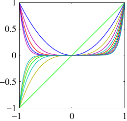
Polynomial

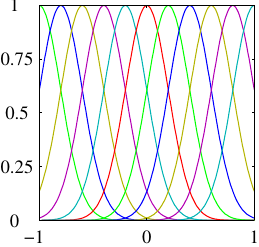
Gaussian
Sigmoid
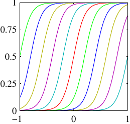
Your data is flat, then jumps to a higher level and stays there. Which of the three captures that step most naturally — and which fights it?

The polynomial of Lecture 0 used \(\phi_j(x)=x^j\). Gaussian/sigmoid bases are local vs. global — the choice is an inductive bias.

Bishop Fig 4.2

Basis ① — Polynomial: a global basis

\[ \phi_j(x) = x^{\,j} \]

  • one curve covers the whole axis — global support
  • so every weight \(w_j\) bends the entire fit at once
  • Purpose: capture a smooth, overall trend with just a few terms
  • knobs: only the degree \(M\) (how many powers)

Downside: a point in one region tugs the curve far away → edge wiggles & wild extrapolation — the polynomial overfitting of Lecture 0.

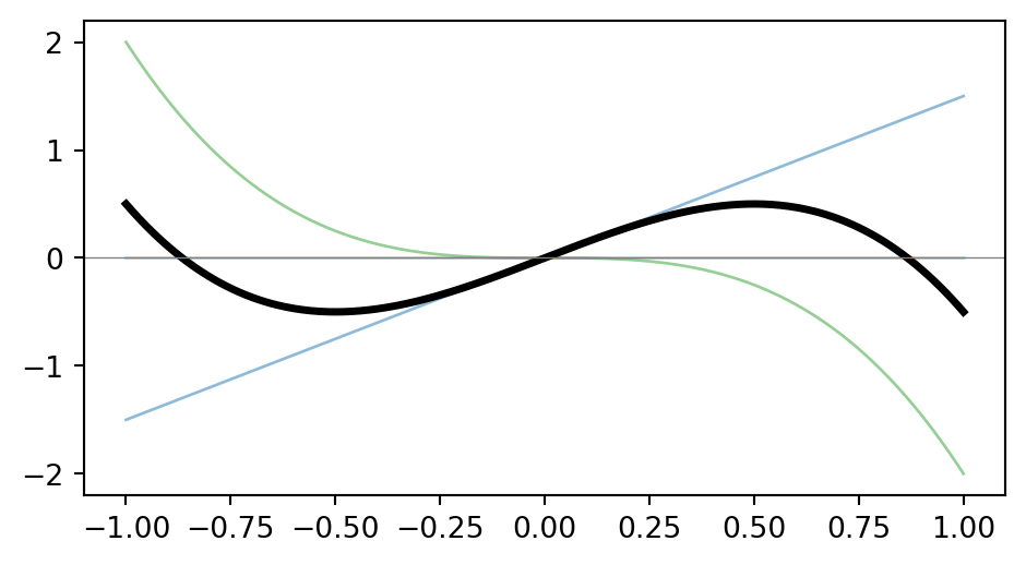
Polynomial — building \(y(x)\)

Weight each faint power \(w_j x^j\), then add → the bold curve \(y(x)\):

\[ y(x, \vw)=\sum_{j=1}^{3} w_j\,x^{\,j} \]

\(\vw=(1.5,\ 0,\ -2)\)

\[ y(x, \vw) =\;1.5x-2x^3 \]

Bias (\(\phi_0=1\)) omitted here for clarity.

\(y=1.5x-2x^3 \Rightarrow y(0.5)=0.75-0.25=\mathbf{0.5}\). Change one coefficient \(w_j\) → the whole curve bends (global support).

Basis ② — Gaussian: a local bump

\[ \phi_j(x) = \exp\!\Big(\!-\frac{(x-\mu_j)^2}{2s^2}\Big) \]

  • a bell centred at \(\mu_j\), width \(s\); ≈ 0 far away — local support
  • weight \(w_j\) = the height of the bump at \(\mu_j\)
  • Purpose: build the curve from local bumps — nearby \(x \Rightarrow\) nearby \(y\)
  • knobs: each centre \(\mu_j\) and the width \(s\) (small = sharp/overfit, large = smooth)

Move one data point → only the nearby bumps react. Local support = stable & controllable — the idea behind RBFs and kernels.

Gaussian — building \(y(x)\)

Stack 4 faint weighted bumps \(w_j\phi_j\) → the bold curve \(y(x)\):
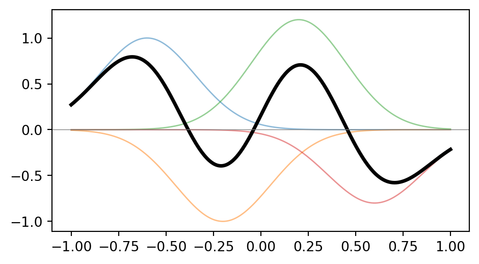
\[ y(x, \vw)=\sum_{j=1}^4 w_j\,e^{-\frac{(x-\mu_j)^2}{2s^2}} \]

\(s=0.25\)

\(\vmu=(-0.6,\,-0.2,\,0.2,\,0.6)\)

\(\vw=(1,\,-1,\,1.2,\,-0.8)\)

Bias (\(\phi_0=1\)) omitted here for clarity.

Each bump acts only near its centre \(\mu_j\) → editing one weight reshapes \(y\) locally. Shrink the width \(s\) and the bumps sharpen — more capacity, more overfitting.

Basis ③ — Sigmoid: a soft threshold

\[ \phi_j(x) = \sigma\!\Big(\frac{x-\mu_j}{s}\Big),\qquad \sigma(a)=\frac{1}{1+e^{-a}} \]

  • a soft step from 0 → 1, switching on at \(\mu_j\) (steepness \(1/s\))
  • Purpose: a switch / threshold — model on–off & saturation
  • two sigmoids subtracted make a bump → can mimic Gaussian locality too

This \(\sigma\) is the neural-net activation: a hidden layer = sigmoid basis whose \(\mu_j,s\) are learned, not chosen by hand → Lecture 5.

Sigmoid — building \(y(x)\)

Stack 3 faint weighted steps \(w_j\,\sigma(\cdot)\) → the bold curve \(y(x)\):
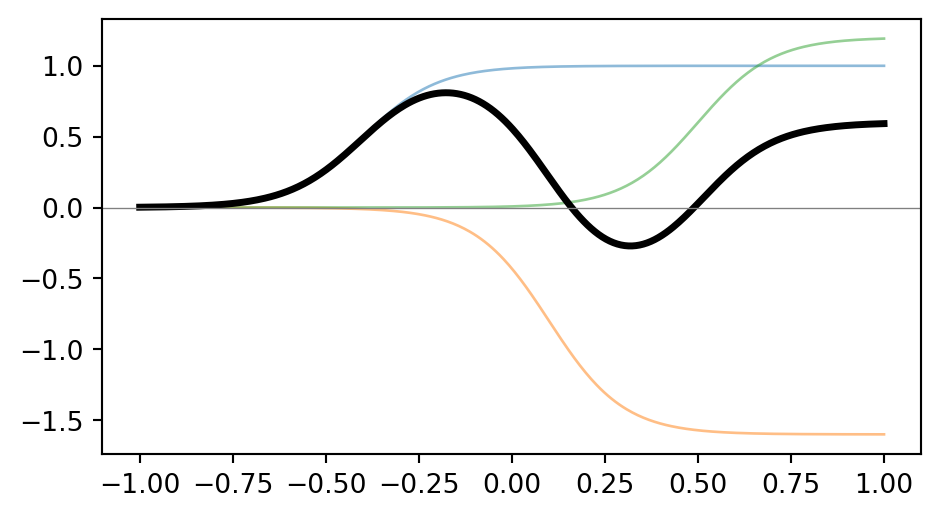
\[ y(x, \vw)=\sum_{j=1}^3 w_j\,\sigma\!\Big(\tfrac{x-\mu_j}{s}\Big) \]

\(s=0.1\)

\(\vmu=(-0.4,\,0.1,\,0.5)\)

\(\vw=(1,\,-1.6,\,1.2)\)

Bias (\(\phi_0=1\)) omitted here for clarity.

Each step switches on at its \(\mu_j\); up- and down-steps stack into plateaus. A hidden layer simply learns these \(\mu_j,\,s,\,w_j\)Lecture 5.

Polynomial, Gaussian, Sigmoid: Same \(\vw\)-and-sum machinery across all three — but the family of curves you can reach is set entirely by the basis.

Basis ④ — ReLU: a piecewise-linear ramp
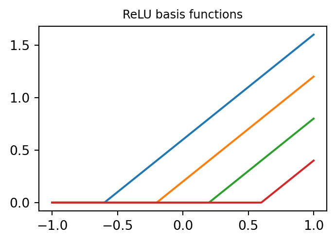
\[ \phi_j(x)=\max(0,\ x-\mu_j)=(x-\mu_j)_+ \]

  • flat 0 until \(\mu_j\), then a straight ramp (slope 1) — a “hinge”
  • Purpose: build piecewise-linear functions; each ReLU adds one kink at \(\mu_j\)
  • vs sigmoid: an unbounded ramp, not a saturating step
  • knobs: the kink location \(\mu_j\) (height/slope via \(w_j\))

The modern default activation: no saturation → gradients don’t vanish for \(x>0\). A ReLU network is a piecewise-linear function approximator → Lecture 5.

Not in Bishop Fig 4.2 — ReLU is the activation most modern deep nets actually use.

ReLU — building \(y(x)\)

Stack 3 faint weighted ramps \(w_j\phi_j\) → the bold, piecewise-linear \(y(x)\):
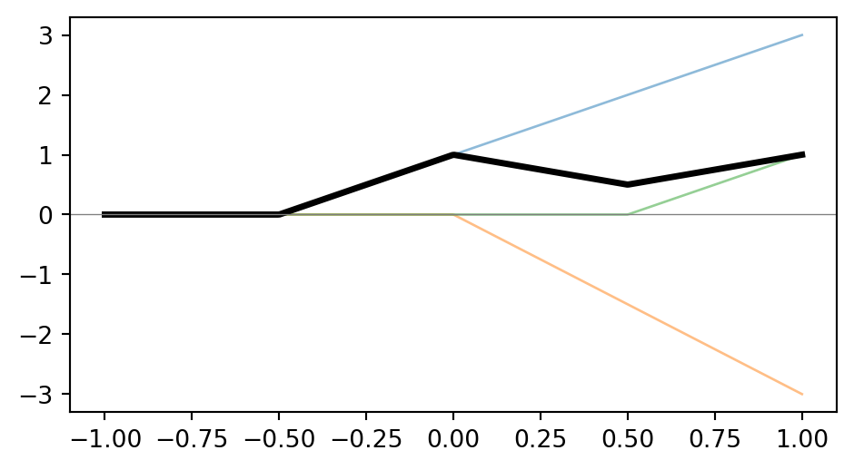
\[ y(x,\vw)=\sum_{j=1}^3 w_j\,\max(0,\,x-\mu_j) \]

\(\vmu=(-0.5,\,0,\,0.5)\)

\(\vw=(2,\,-3,\,2)\)

Bias (\(\phi_0=1\)) omitted here for clarity.

At \(x=0\) only the first ramp is on: \(y(0)=2(0.5)-3(0)+2(0)=\mathbf{1}\). Each ReLU adds a kink (slope change) at its \(\mu_j\) → the curve is piecewise-linear.

ReLU joins the family: same \(\vw\)-and-sum machinery, but the curves are piecewise-linear — and this is the basis modern deep nets actually use → Lecture 5.

This is a single-layer network
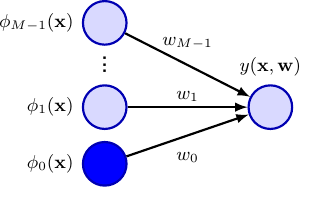
\[ y(\vx,\vw) = \sum_{j=0}^{M-1} w_j\,\phi_j(\vx) \]

  • The basis functions \(\phi_j\) are fixed features
  • The output is a weighted sum — a single layer of weights \(\vw\)

Deep learning’s big idea (later): learn the features \(\phi_j\) instead of fixing them by hand.

Bishop Fig 4.1

Part 2 · Least Squares

A tiny fit to start

Three points that are not on a straight line: \[(x,t):\quad (0,1),\ (1,3),\ (2,2)\]

We will fit a line \(y = w_0 + w_1 x\) by least squares.

The line can’t pass through all three points — so where does least squares put it? Guess: is the slope \(w_1\) positive, negative, or zero? And will the three residuals \(t_n - y(x_n)\) add up to zero?

The sum-of-squares loss

Given data \(\{(\vx_n, t_n)\}_{n=1}^N\), measure misfit by:

\[ E_D(\vw) = \frac{1}{2}\sum_{n=1}^{N}\big\{ t_n - \vw^{\mathsf T}\boldsymbol{\phi}(\vx_n) \big\}^2 \]

Collect the data into the design matrix \(\boldsymbol{\Phi}\in\R^{N\times M}\) with \(\Phi_{nj}=\phi_j(\vx_n)\):

\[\boldsymbol{\Phi}=\begin{bmatrix} \phi_0(\vx_1) & \phi_1(\vx_1) & \cdots & \phi_{M-1}(\vx_1)\\ \phi_0(\vx_2) & \phi_1(\vx_2) & \cdots & \phi_{M-1}(\vx_2)\\ \vdots & \vdots & \ddots & \vdots\\ \phi_0(\vx_N) & \phi_1(\vx_N) & \cdots & \phi_{M-1}(\vx_N) \end{bmatrix}\]

Then the loss becomes simply:

\[ E_D(\vw) = \tfrac{1}{2}\,\norm{\vt - \boldsymbol{\Phi}\vw}^2 \]

\(E_D\) is quadratic in \(\vw\) ⇒ a single global minimum, found in closed form.

The normal equations

Set the gradient to zero:

\[ \nabla_{\vw} E_D = -\,\boldsymbol{\Phi}^{\mathsf T}\big(\vt - \boldsymbol{\Phi}\vw\big) = 0 \]

\[ \boldsymbol{\Phi}^{\mathsf T}\boldsymbol{\Phi}\,\vw = \boldsymbol{\Phi}^{\mathsf T}\vt \quad\Longrightarrow\quad \boxed{\;\vw_{\mathrm{ML}} = \big(\boldsymbol{\Phi}^{\mathsf T}\boldsymbol{\Phi}\big)^{-1}\boldsymbol{\Phi}^{\mathsf T}\vt = \boldsymbol{\Phi}^{\dagger}\vt\;}\]

\(\boldsymbol{\Phi}^{\dagger}\) is the Moore–Penrose pseudo-inverse — exactly what np.linalg.lstsq computes.

Worked example: solve the tiny fit

Basis \(\boldsymbol\phi(x)=[1,\ x]^{\mathsf T}\), so for \((0,1),(1,3),(2,2)\): \[\boldsymbol\Phi=\begin{bmatrix}1&0\\1&1\\1&2\end{bmatrix},\qquad \vt=\begin{bmatrix}1\\3\\2\end{bmatrix}\]

\[\boldsymbol\Phi^{\mathsf T}\boldsymbol\Phi=\begin{bmatrix}3&3\\3&5\end{bmatrix},\qquad \boldsymbol\Phi^{\mathsf T}\vt=\begin{bmatrix}6\\7\end{bmatrix}\] Solve \(\boldsymbol\Phi^{\mathsf T}\boldsymbol\Phi\,\vw=\boldsymbol\Phi^{\mathsf T}\vt\) (determinant \(=6\)): \[\vw_{\mathrm{ML}}=\frac{1}{6}\begin{bmatrix}5&-3\\-3&3\end{bmatrix}\begin{bmatrix}6\\7\end{bmatrix} =\frac{1}{6}\begin{bmatrix}9\\3\end{bmatrix}=\begin{bmatrix}1.5\\0.5\end{bmatrix}\] Line \(y=1.5+0.5x\) → predictions \(1.5,\,2.0,\,2.5\); residuals \(-0.5,\,+1.0,\,-0.5\) (sum \(=0\) ✓).

Slope is positive (\(w_1=0.5\)) and the residuals cancel — forced by the all-ones column of \(\boldsymbol\Phi\). Did your prediction match?

Your turn

Same recipe, new data. Fit \(y=w_0+w_1 x\) by least squares to: \[(0,1),\ (1,2),\ (2,0)\]

  1. Write the design matrix \(\boldsymbol\Phi\) and target \(\vt\).
  2. Form \(\boldsymbol\Phi^{\mathsf T}\boldsymbol\Phi\) and \(\boldsymbol\Phi^{\mathsf T}\vt\).
  3. Solve for \(\vw_{\mathrm{ML}}\), then check the residuals sum to zero.

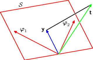
Least squares is a projection

  • \({\vt}\) lives in \(\R^N\); the reachable predictions \(\boldsymbol{\Phi}\vw\) span a subspace \(\mathcal S\)
  • Least squares picks \(\vy=\boldsymbol{\Phi}\vw_{\mathrm{ML}}\) = the orthogonal projection of \(\vt\) onto \(\mathcal S\)
  • The residual \(\vt-\vy\) is ⟂ to \(\mathcal S\) → that is the normal equations
  • จากรูป: \(N=3\) samples, \(M=2\) พารามิเตอร์ → \(\mathcal{S}\) เป็นระนาบ 2D plane ใน 3D space

Bishop Fig 4.3 — geometric view of least squares

Subspace \(\mathcal{S}\)

\(\boldsymbol{\Phi}\) คือเมทริกซ์ขนาด \(N\times M\) ที่ตายตัว (เป็นข้อมูล) แต่ \(\vw\in\mathbb{R}^M\) เปลี่ยนได้:

\[\boldsymbol{\Phi}\vw = w_0\underbrace{\boldsymbol{\phi}_0}_{\text{col 0}} + w_1\underbrace{\boldsymbol{\phi}_1}_{\text{col 1}} + \cdots + w_{M-1}\underbrace{\boldsymbol{\phi}_{M-1}}_{\text{col }M-1}\in\mathcal{S}\subseteq \mathbb{R}^N\]

โดยที่ \(\boldsymbol{\phi}_j=[\phi_j(\vx_1),\,\phi_j(\vx_2),\,\ldots,\,\phi_j(\vx_N)]^\top\in\mathbb{R}^N\) คือคอลัมน์ที่ \(j\) ของ \(\boldsymbol{\Phi}\)

เซตของทุก prediction ที่เป็นไปได้ = column space ของ \(\boldsymbol{\Phi}\) (Linear combination ของคอลัมน์ของ \(\boldsymbol{\Phi}\))

  • ปกติ \(N\gg M\) (ข้อมูลมากกว่าพารามิเตอร์) → subspace \(\mathcal{S}\) มีมิติ \(\leq M\) แต่อยู่ใน \(\mathbb{R}^N\) ดังนั้น \(\vt\) เกือบแน่นอนที่จะไม่อยู่ใน \(\mathcal{S}\)

Two extensions: online & multi-output

Sequential learning (§4.1.5) — the closed form needs all data at once. Update one point at a time instead: \[\vw^{(\tau+1)}=\vw^{(\tau)}+\eta\big(t_n-\vw^{(\tau)\mathsf T}\boldsymbol\phi_n\big)\boldsymbol\phi_n\] - “error × input” again — this is (stochastic) gradient descent (L6), and the rule behind training on huge / streaming data

Multiple outputs (§4.1.7) — for a vector target \(\vt\in\R^K\), stack a weight matrix \(W\):
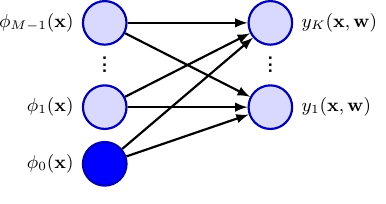
\[W_{\mathrm{ML}}=\big(\boldsymbol\Phi^{\mathsf T}\boldsymbol\Phi\big)^{-1}\boldsymbol\Phi^{\mathsf T}\mathbf{T}\] - the same \(\boldsymbol\Phi^\dagger\) solves every output column independently — one fit, \(K\) predictions

Bishop Fig 4.4

Part 3 · Why Squared Error? The Probabilistic View

A noise model

Assume the target is the function plus Gaussian noise:

\[ t = y(\vx,\vw) + \varepsilon, \qquad \varepsilon \sim \mathcal N(0, \beta^{-1}) \]

Equivalently, a conditional distribution over \(t\):

\[ p(t \given \vx, \vw, \beta) = \mathcal N\!\big(t \;\big|\; y(\vx,\vw),\; \beta^{-1}\big) = \mathcal N\!\big(t \;\big|\; \vw^{\mathsf T}\boldsymbol{\phi}(\vx),\; \beta^{-1}\big) \]

\(\beta = 1/\sigma^2\) is the precision (inverse variance).

Theory pillar LLMs gloss over: where the squared-error loss actually comes from

Maximum likelihood Estimation

Assuming i.i.d. data, the likelihood is

\[ p(\vt \given \boldsymbol{\Phi}, \vw, \beta) = \prod_{n=1}^{N} \mathcal N\!\big(t_n \given \vw^{\mathsf T}\boldsymbol{\phi}(\vx_n),\, \beta^{-1}\big) \]

Take the log:

\[ \ln p(\vt\given\vw,\beta) = \frac{N}{2}\ln\beta - \frac{N}{2}\ln(2\pi) \;-\; \beta\,\underbrace{\tfrac{1}{2}\textstyle\sum_n\{t_n-\vw^{\mathsf T}\boldsymbol{\phi}(\vx_n)\}^2}_{=\,E_D(\vw)} \]

Squared error is not arbitrary — it is the MLE under Gaussian noise.

The noise assumption chooses the loss

Gaussian noise → squared loss (just derived)

\[p(t\given\vx)\propto e^{-\frac{\beta}{2}(t-y)^2}\]

\[-\ln p \;\propto\; \underbrace{\sum_n(t_n-y_n)^2}_{\text{L2 loss}}\]

Optimal point prediction: mean \(\E[t|\vx]\)

Laplacian noise → absolute loss

\[p(t\given\vx)\propto e^{-|t-y|/b}\]

\[-\ln p \;\propto\; \underbrace{\sum_n|t_n-y_n|}_{\text{L1 loss}}\]

Optimal point prediction: median of \(p(t|\vx)\)

The loss function is not chosen arbitrarily — it is implied by your belief about how noise behaves. Change the noise model, and the loss changes with it.

Laplacian is heavier-tailed than Gaussian → L1 regression is more robust to outliers.

Solving, and predicting

Maximizing over \(\vw\) gives the same normal equations:

\[ \vw_{\mathrm{ML}} = \big(\boldsymbol{\Phi}^{\mathsf T}\boldsymbol{\Phi}\big)^{-1}\boldsymbol{\Phi}^{\mathsf T}\vt \]

And over \(\beta\):

\[ \frac{1}{\beta_{\mathrm{ML}}} = \frac{1}{N}\sum_{n=1}^{N}\big\{t_n-\vw_{\mathrm{ML}}^{\mathsf T}\boldsymbol{\phi}(\vx_n)\big\}^2 \]

We don’t just get a point prediction but a distribution:

\[ p(t\given\vx) = \mathcal N\!\big(t \given \vw_{\mathrm{ML}}^{\mathsf T}\boldsymbol{\phi}(\vx),\, \beta_{\mathrm{ML}}^{-1}\big) \]

→ predictions come with a notion of uncertainty (revisited in Trustworthy AI).

From distribution to a single prediction
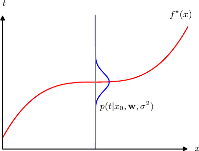
The noise model gives us a full distribution at every \(x\):

\[p(t \given x) = \mathcal{N}(t \mid y(x,\vw),\, \beta^{-1})\]

The red curve \(f^\star(x)\) is the underlying truth; the blue bell at \(x_0\) shows how noisy observations scatter around it.

In practice we must commit to one number — a point prediction. The distribution alone is not enough.

Which single number should we report from \(p(t|x)\)? The mean, the mode, or something else — and does it depend on the loss we care about?

Bishop Fig 4.5

The optimal prediction: conditional mean

Decision theory (§4.2): define \(L=(y(\vx)-t)^2\) and find \(y(\vx)\) that minimises expected loss over all \((\vx,t)\):

\[\E[L]=\iint \big(y(\vx)-t\big)^2\, p(\vx,t)\,dt\,d\vx\]

Expand and minimise pointwise for each \(\vx\):

\[\frac{\partial\,\E[L]}{\partial\,y(\vx)} = 0 \;\Longrightarrow\; \boxed{y^\star(\vx)=\E[t\given\vx]}\]

The optimal point prediction under squared loss is the conditional mean — not a heuristic, a theorem.

Why this matters: \(h(\vx)=\E[t|\vx]\) is the ceiling no model can beat — bias–variance (L4) decomposes how far your model sits below it. And from L1: the mean minimises \(\E[(X-c)^2]\), so this result is that same fact applied to regression.

Part 4 · Regularization & Wrap-up

Regularized least squares

Add the penalty from Lecture 0:

\[ E(\vw) = \tfrac{1}{2}\norm{\vt-\boldsymbol{\Phi}\vw}^2 + \tfrac{\lambda}{2}\norm{\vw}^2 \]

Still closed-form — just add \(\lambda\mathbf I\):

\[ \boxed{\;\vw = \big(\lambda\mathbf I + \boldsymbol{\Phi}^{\mathsf T}\boldsymbol{\Phi}\big)^{-1}\boldsymbol{\Phi}^{\mathsf T}\vt\;}\]

Derive the boxed solution. Start from \(E(\vw)=\tfrac{1}{2}\norm{\vt-\boldsymbol{\Phi}\vw}^2+\tfrac{\lambda}{2}\norm{\vw}^2\), take \(\nabla_\vw E=0\), and solve for \(\vw\). (Hint: compare with the normal equations — only one term changes.)

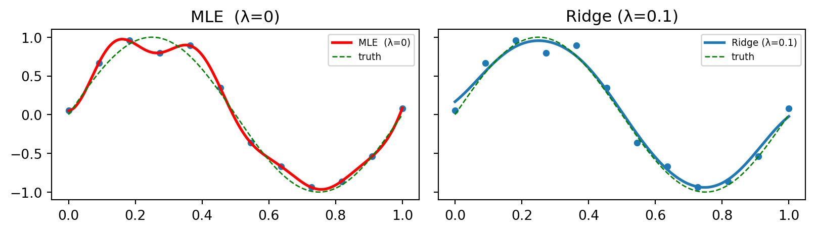
This is ridge regression. Probabilistically it is MAP estimation with a Gaussian prior \(p(\vw)=\mathcal N(\vw\given 0,\,\alpha^{-1}\mathbf I)\), where \(\lambda=\alpha/\beta\) — regularization = a prior belief that weights are small.

🔬 Demo: Gaussian basis + regularization

How is the design matrix defined here? Which basis family is this? What do you expect ridge (\(\lambda>0\)) to do to the fit near the data edges?

import numpy as np, matplotlib.pyplot as plt
rng = np.random.default_rng(1)
x = np.linspace(0, 1, 12); t = np.sin(2*np.pi*x) + 0.15*rng.standard_normal(x.size)
mu, s = np.linspace(0, 1, 9), 0.12
def basis(z): return np.hstack([np.ones((z.size,1)), np.exp(-0.5*((z[:,None]-mu)/s)**2)])
Phi = basis(x); xs = np.linspace(0, 1, 200); truth = np.sin(2*np.pi*xs)
w_mle   = np.linalg.lstsq(Phi, t, rcond=None)[0]           # MLE  (λ = 0)
lam = 0.1
w_ridge = np.linalg.solve(lam*np.eye(Phi.shape[1]) + Phi.T@Phi, Phi.T@t)  # ridge
fig, ax = plt.subplots(1, 2, figsize=(8.5, 2.5), sharey=True)
for a, w, label, color in [(ax[0], w_mle, f"MLE  (λ=0)", "r"),
                            (ax[1], w_ridge, f"Ridge (λ={lam})", "C0")]:
    a.plot(x, t, "o", ms=4); a.plot(xs, basis(xs)@w, color, lw=2, label=label)
    a.plot(xs, truth, "g--", lw=1, label="truth"); a.legend(fontsize=7); a.set_title(label)
plt.tight_layout(); plt.show()
Summary

  1. Linear basis function models \(y=\vw^{\mathsf T}\boldsymbol{\phi}(\vx)\) are nonlinear in \(\vx\) but linear in \(\vw\) → a single-layer network
  2. Least squares has a closed form (normal equations) and a clean projection geometry
  3. Squared error is the maximum-likelihood solution under Gaussian noise — and ridge = a Gaussian prior

📌 Read before next class

Bishop & Bishop (2024), Chapter 5Single-layer Networks: Classification

We move from predicting numbers to predicting classes: logistic regression, softmax, and the cross-entropy loss (its own maximum-likelihood story).

Figures from Bishop & Bishop, Deep Learning: Foundations and Concepts (2024), Chapter 4 — https://www.bishopbook.com/

⌂ Home