\( \newcommand{\vw}{\mathbf{w}} \newcommand{\vx}{\mathbf{x}} \newcommand{\vt}{\mathbf{t}} \newcommand{\vy}{\mathbf{y}} \newcommand{\vz}{\mathbf{z}} \newcommand{\vq}{\mathbf{q}} \newcommand{\vk}{\mathbf{k}} \newcommand{\vv}{\mathbf{v}} \newcommand{\vc}{\mathbf{c}} \newcommand{\vp}{\mathbf{p}} \newcommand{\vh}{\mathbf{h}} \newcommand{\vmu}{\boldsymbol{\mu}} \newcommand{\vsigma}{\boldsymbol{\sigma}} \newcommand{\vepsilon}{\boldsymbol{\epsilon}} \newcommand{\R}{\mathbb{R}} \newcommand{\E}{\mathbb{E}} \newcommand{\norm}[1]{\lVert #1 \rVert} \newcommand{\given}{\,\vert\,} \)

Lecture 19 — Latent Variable Models & EM

Deep Learning · Clustering, GMMs, Expectation–Maximization

Kasemsit Teeyapan

Department of Computer Engineering, Chiang Mai University

Today

  1. Unsupervised learning: structure from data with no labels
  2. K-means — hard clustering
  3. Gaussian mixture models — soft, probabilistic clustering with latent variables
  4. Expectation–Maximization (EM) — the algorithm that fits them
  5. EM = coordinate ascent on the ELBO (L12) — the bridge to VAEs

Reference: Bishop & Bishop (2024), Chapter 15Discrete Latent Variables

Recap → latent variables

A latent variable \(\vz\) is an unobserved cause that explains the data \(\vx\):

\[p(\vx)=\sum_{\vz} p(\vx\given\vz)\,p(\vz)\]

  • which cluster a point came from
  • what digit a handwriting image is
  • the hidden code in a VAE (L12)

We never see \(\vz\). If we knew it, fitting would be easy; if we knew the parameters, inferring \(\vz\) would be easy. Chicken-and-egg → EM.

K-means clustering

Partition data into \(K\) clusters; alternate two steps:

  1. assign each point to its nearest center \(\vmu_k\)
  2. update each center to the mean of its points

Minimizes within-cluster squared distance. Always converges (to a local optimum).

K-means makes a hard choice — each point belongs to exactly one cluster. But points near a boundary are ambiguous; we’d like to express that uncertainty.

Gaussian mixture models

Model the data as a mixture of \(K\) Gaussians:

\[p(\vx)=\sum_{k=1}^{K}\pi_k\,\mathcal N(\vx\given\vmu_k,\Sigma_k)\]

  • \(\pi_k\) = mixing weight (prior \(p(z_k{=}1)\)), \(\sum_k\pi_k=1\)
  • the latent \(\vz\) = which component generated \(\vx\)

Responsibility = posterior over clusters (soft assignment):

\[\gamma_{nk}=p(z_k{=}1\given\vx_n)=\frac{\pi_k\,\mathcal N(\vx_n\given\vmu_k,\Sigma_k)}{\sum_j \pi_j\,\mathcal N(\vx_n\given\vmu_j,\Sigma_j)}\]

The EM algorithm

E-step — with current params, compute responsibilities: \[\gamma_{nk}=p(z_k{=}1\given\vx_n)\]

M-step — with responsibilities fixed, re-fit by weighted MLE: \[\vmu_k=\frac{\sum_n \gamma_{nk}\vx_n}{N_k},\quad \pi_k=\frac{N_k}{N},\quad N_k=\sum_n\gamma_{nk}\]

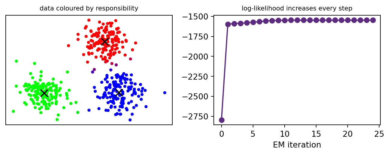
Pillar: EM breaks the chicken-and-egg by alternating — guess \(\vz\) (E), re-fit params (M), repeat. Each round never decreases the likelihood.

🔬 Demo: EM fits a mixture

import numpy as np, matplotlib.pyplot as plt
rng = np.random.default_rng(1)
X = np.vstack([rng.normal(m, 0.8, (150,2)) for m in ([0,0],[4,4],[5,0])]); N, K = len(X), 3
mu = X[rng.choice(N,K,replace=False)]; cov = np.array([np.eye(2)]*K); pi = np.ones(K)/K
def g(X,m,c): d=X-m; return np.exp(-0.5*np.sum(d@np.linalg.inv(c)*d,1))/np.sqrt((2*np.pi)**2*np.linalg.det(c))
lls=[]
for _ in range(25):
    R = np.stack([pi[k]*g(X,mu[k],cov[k]) for k in range(K)],1)            # E-step
    lls.append(np.sum(np.log(R.sum(1)))); R /= R.sum(1,keepdims=True)
    Nk = R.sum(0); mu = (R.T@X)/Nk[:,None]                                  # M-step
    for k in range(K): d=X-mu[k]; cov[k]=(R[:,k,None]*d).T@d/Nk[k]+1e-6*np.eye(2)
    pi = Nk/N
fig,ax=plt.subplots(1,2,figsize=(6.8,2.8))
ax[0].scatter(X[:,0],X[:,1],c=R,s=8); ax[0].scatter(mu[:,0],mu[:,1],c="k",marker="x",s=80)
ax[0].set_title("data coloured by responsibility",fontsize=8); ax[0].set_xticks([]); ax[0].set_yticks([])
ax[1].plot(lls,"o-",color="#5d2c80"); ax[1].set_title("log-likelihood increases every step",fontsize=8)
ax[1].set_xlabel("EM iteration"); plt.tight_layout(); plt.show()
EM = climbing the ELBO

Same ELBO as the VAE (L12), for any \(q(\vz)\): \[\ln p(\vx)=\underbrace{\E_q\!\Big[\ln\tfrac{p(\vx,\vz)}{q(\vz)}\Big]}_{\mathcal L(q,\theta)}+\mathrm{KL}\big(q\,\Vert\,p(\vz\given\vx)\big)\]

  • E-step: set \(q=p(\vz\given\vx)\) → KL\(=0\), so \(\mathcal L\) touches \(\ln p(\vx)\)
  • M-step: maximize \(\mathcal L\) over \(\theta\)

Pillar: EM is coordinate ascent on the ELBO — E optimizes \(q\), M optimizes \(\theta\). A VAE is the same idea when the posterior is intractable: replace the exact E-step with a neural encoder (amortized inference).

K-means is a limit of GMM

Take a GMM with \(\Sigma_k=\varepsilon I\) and let \(\varepsilon\to 0\):

  • responsibilities \(\gamma_{nk}\to\) hard 0/1 (nearest center wins)
  • E-step → assignment; M-step → mean update

That’s exactly K-means.

K-means = “hard EM.” GMM keeps the uncertainty (soft responsibilities) that K-means throws away — and gives a full probability model \(p(\vx)\) you can sample from.

Summary

  1. Latent variables \(\vz\) explain data we can’t fully observe: \(p(\vx)=\sum_z p(\vx\given\vz)p(\vz)\)
  2. GMM = soft, probabilistic clustering; responsibilities = posterior \(p(\vz\given\vx)\)
  3. EM alternates E (infer \(\vz\)) and M (refit \(\theta\)); likelihood never decreases
  4. EM = coordinate ascent on the ELBO — exactly the VAE objective (L12)
  5. K-means = hard-assignment limit of a GMM

Something to think about: EM only guarantees a local optimum, and is sensitive to initialization. Why is running it from several random starts (or K-means init) standard practice?

📌 Connections

EM (this lecture) and variational inference / VAEs (L12) optimize the same ELBO. When the E-step posterior is intractable, we either approximate it (VAE encoder) or sample it — the subject of the next lecture.

References: Dempster, Laird & Rubin, Maximum Likelihood from Incomplete Data via the EM Algorithm (1977). Figures/derivations from Bishop & Bishop (2024), Ch 15 — https://www.bishopbook.com/

⌂ Home