umbrella, given it rained:\(p(\text{umb}\given\text{rain})=\frac{30}{40}=0.75\) — only look at rain days
Every probability was a fraction of counts. And notice the pattern: \(\;0.3 = 0.75\times 0.4\), i.e. \(\;p(\text{rain},\text{umb}) = p(\text{umb}\given\text{rain})\,p(\text{rain})\).
The same pattern, in general
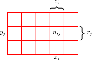
Replace numbers with counts \(n_{ij}\) in a grid of \(N\) trials; column total \(c_i=\sum_j n_{ij}\).
The same three fractions, now general:
joint\(\;p(x_i,y_j)=\dfrac{n_{ij}}{N}\)
marginal\(\;p(x_i)=\dfrac{c_i}{N}=\sum_j p(x_i,y_j)\) → sum rule
Everything distills to two rules — these are the whole foundation:
Sum rule(marginalize)\[p(X)=\sum_Y p(X,Y)\] add over the variable you don’t care about
Product rule(factorize)\[p(X,Y)=p(Y\given X)\,p(X)\] a joint = conditional \(\times\) marginal
All of probabilistic modelling — likelihoods, Bayes’ theorem, marginalizing latent variables in deep models — is built from just these two. Worth memorizing.
One more relation: independence
The product rule always holds: \(\;p(X,Y)=p(Y\given X)\,p(X)\).
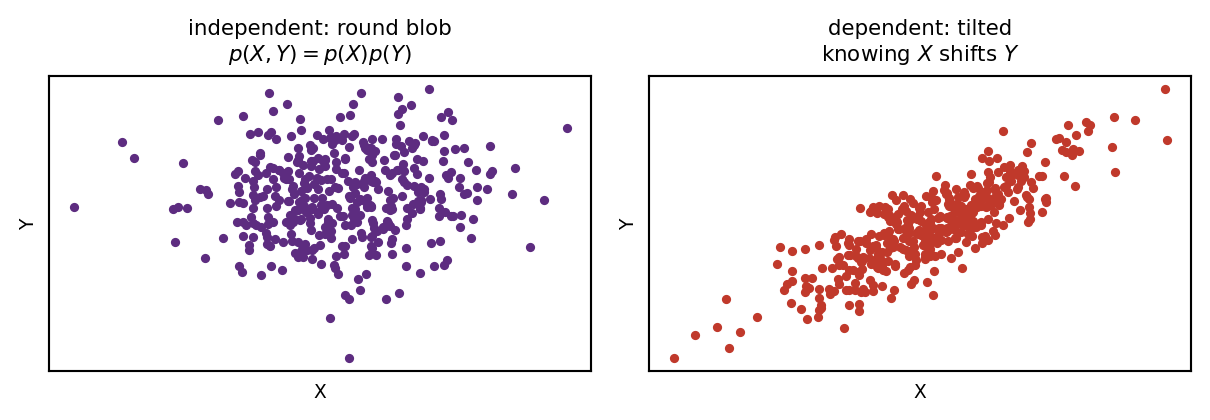
Independence is the special case where conditioning changes nothing — knowing one tells you nothing about the other, \(p(Y\given X)=p(Y)\) — so the product rule collapses to a plain product:
\[X \perp Y \iff p(Y\given X)=p(Y) \iff p(X,Y)=p(X)\,p(Y)\]
Back to our toy:\(p(\text{umb})=0.5\) but \(p(\text{umb}\given\text{rain})=0.75\neq0.5\) → rain & umbrella are dependent (right) — exactly why a model can learn one from the other. The i.i.d. assumption (L4) is that training points are independent, letting us multiply per-point likelihoods (MLE, later in this deck).
A medical test: two ways to be right
The question. A disease affects only 1 in 100 people. A test is 90% sensitive and 90% specific. You take the test and it comes back positive — what is the probability that you actually have the disease? (Any guess?)
First, what do “90% sensitive” and “90% specific” mean? Run the test on people whose status we already know → four outcomes:
sick
healthy
test +
✅ TP
❌ FP
test −
❌ FN
✅ TN
sensitivity\(=p(+\given\text{sick})\) — of sick people, how many caught? Here 90% (so 10% missed)
specificity\(=p(-\given\text{healthy})\) — of healthy people, how many cleared? Here 90% (so 10% false alarms)
“90 / 90” sounds great — but on healthy people it still raises a false alarm 10% of the time. Hold that thought.
Bayes in action: count 10,000 people
Back to the question: the disease is rare (1%), the test is 90% sensitive and 90% specific, and yours came back positive. Are you actually sick? Instead of a formula, let’s just count people.
Count 10,000 people:
1% sick → 100 sick, 9,900 healthy
of the 100 sick: \(0.9\times100=\)90 test positive (10 missed)
of the 9,900 healthy: \(0.1\times9900=\)990 test positive (false alarms)
Notice what we did: reversed the conditional, from \(p(+\given\text{sick})\) to \(p(\text{sick}\given +)\). Is there a formula for that? → next.
Only ~8% — the prior (rarity) dominates. Same arithmetic appears as precision under class imbalance in ML.
Bayes’ theorem
That reversal — going from \(p(+\given\text{sick})\) to \(p(\text{sick}\given +)\) — is Bayes’ theorem. It drops out of the product rule written two ways:
\(\text{posterior}\propto\text{likelihood}\times\text{prior}\) — Bayes is just the two rules combined, yet it is the engine for reversing conditionals and updating belief from data.
🔬 Demo: Bayes by simulation
import numpy as nprng = np.random.default_rng(0) # rng.random(n) = n draws from Uniform[0,1) (same as rng.uniform(0,1,n))N =1_000_000disease = rng.random(N) <0.01# 1% prevalence (the prior)positive = np.empty(N, bool)positive[disease] = rng.random(disease.sum()) <0.90# sick → 90% test positive (sensitivity)positive[~disease] = rng.random((~disease).sum()) <0.10# healthy → 10% test positive (false alarm)print("P(disease | positive) ≈", round(disease[positive].mean(), 3))
P(disease | positive) ≈ 0.083
Simulating a million people lands on ~0.083 — exactly the Bayes calculation. Code confirms the theory.
Bayes’ theorem = how to learn from data
Infer the model parameters\(\vw\) from the observed dataset\(\mathcal D=\{(\vx_n,t_n)\}\).
Prior\(p(\vw)\) — what we believe about model parameters before seeing data
Likelihood\(p(\mathcal D\given\vw)\) — how well parameters explain the data
Posterior\(p(\vw\given\mathcal D)\) — updated belief after data
This single equation is the backbone behind MLE, MAP, and regularization — we use it today and all term
Probability densities
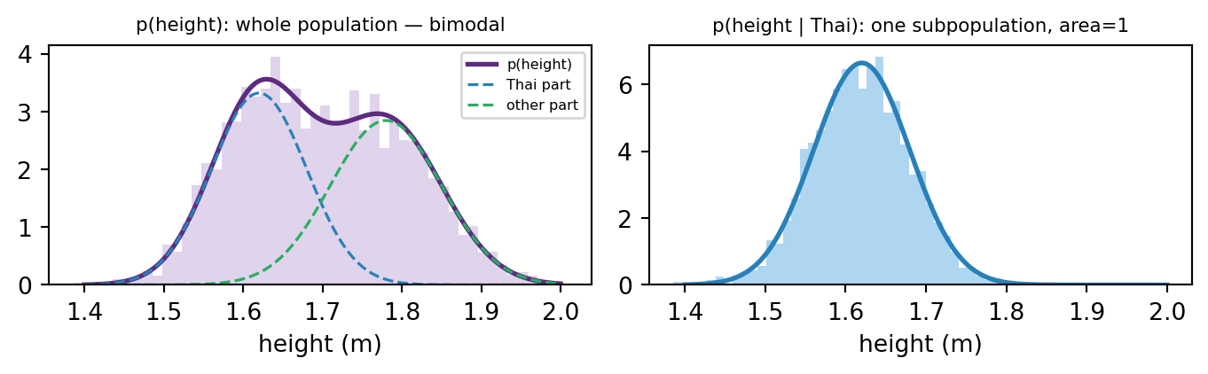
How tall is a random person? A mixed population gives a multimodal density \(p(x)\) (left). Conditioning on a subgroup — given Thai — keeps one slice and renormalizes (right): the continuous version of “only rain days”.
conditioning = keep one subpopulation, then rescale so the area is 1 again (note the right curve is taller)
area (not height) is probability; a density can exceed 1 (≈6/m), and \(p(\text{exact value})=0\) — only ranges count
The same idea in 2D: counts → a surface
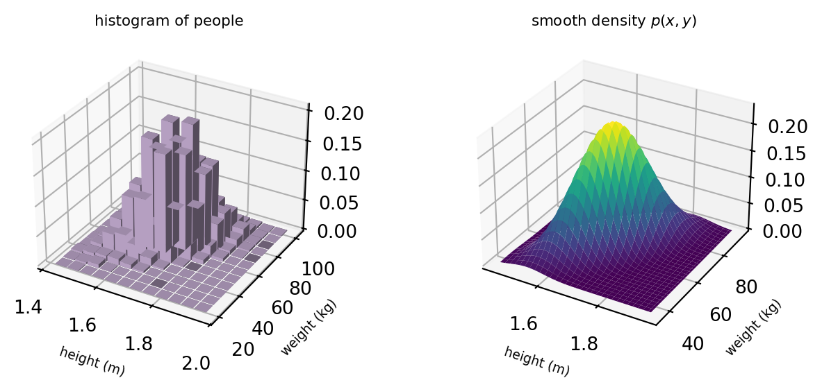
Now take height and weight together → a density over two variables, a surface\(p(x,y)\). Taller people tend to weigh more, so the cloud tilts (correlation). (Volume under the surface = 1.)
Beyond 2D: a density over \(D\) variables is the same idea — we just can’t draw it past 3D. In deep learning \(\vx\) often lives in thousands of dimensions (e.g. pixels); the sum / product / Bayes rules still hold exactly (sums → integrals).
Expectations and variance
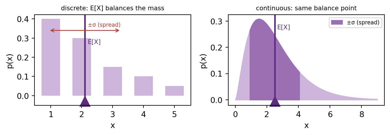
Expectation\(\E[X]=\sum_x p(x)\,x\) (or \(\int p(x)\,x\,dx\)) = the balance point (center of mass) of the probability mass. Variance\(\mathrm{var}[X]=\E[(X-\E X)^2]\) = how widely the mass is spread. (Fair die → \(\E[X]=3.5\).)
Why we care: every loss is an expectation (“average over the data”). Covariance\(\E[(x-\bar x)(y-\bar y)]\) extends this — do two variables move together?
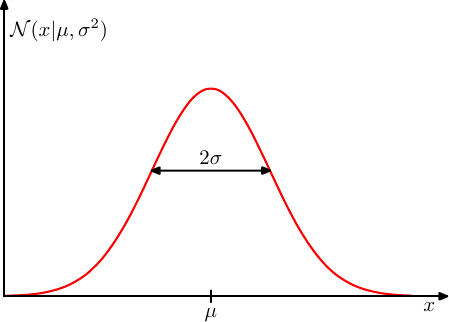
our noise model for regression — the most important distribution in the course
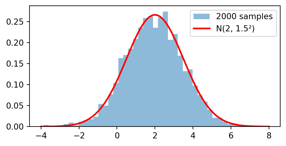
Why is it everywhere? Add up many small independent random effects and the total is always bell-shaped (the Central Limit Theorem). Measurement noise, heights, exam scores — all roughly Gaussian.
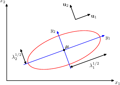
Intuition: a bell in 2D — \(\boldsymbol\mu\) centers the cloud, \(\boldsymbol\Sigma\)stretches & tilts it (diagonal = independent axes, off-diagonal = correlation)
contours of constant density are ellipses: axes = eigenvectors of \(\boldsymbol\Sigma\), widths \(\propto\sqrt{\lambda_i}\)
Bishop Fig 3.3 (§3.2.1, geometry of the Gaussian)
Transforming a density: mind the stretch
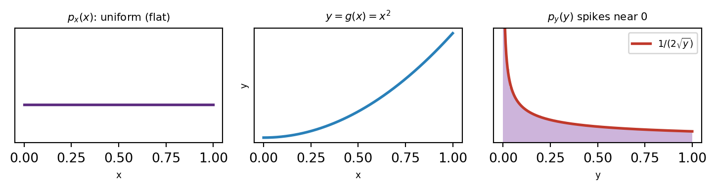
Push a random variable through \(y=g(x)\). Probability mass is conserved, so the density must rescale by how much \(g\)stretches space:
The input is flat, yet \(p_y\)spikes near 0 — because \(g=x^2\) is flat there (\(g'(0)=0\)), so points pile up; where \(g\) is steep, mass thins. The simulated histogram matches the exact \(|dx/dy|=1/(2\sqrt y)\). This Jacobian rule is the engine of normalizing flows and change-of-variables in diffusion/VAE (L12). (A density’s peak is not transform-invariant — unlike an expectation.)
Bishop §2.4 — transformation of densities
Maximum likelihood estimation
Idea: choose parameters that make the observed data most probable.
Toy: flip a coin 10 times, see 7 heads. The bias \(p\) that makes “7 heads” most likely is just \(\hat p=\tfrac{7}{10}\) — the fraction. That’s MLE.
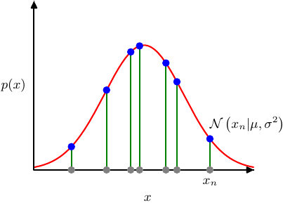
For a Gaussian, it gives the equally intuitive answers: \[ \mu_{\mathrm{ML}} = \tfrac{1}{N}\textstyle\sum_n x_n, \quad \sigma^2_{\mathrm{ML}} = \tfrac{1}{N}\textstyle\sum_n (x_n-\mu_{\mathrm{ML}})^2 \]
We take the log to turn products into sums — the trick behind the least-squares derivation (L2).
Bishop Fig 2.9 (§2.3.3)
Bias of maximum likelihood
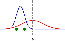
MLE is powerful but not perfect — it underestimates the variance:
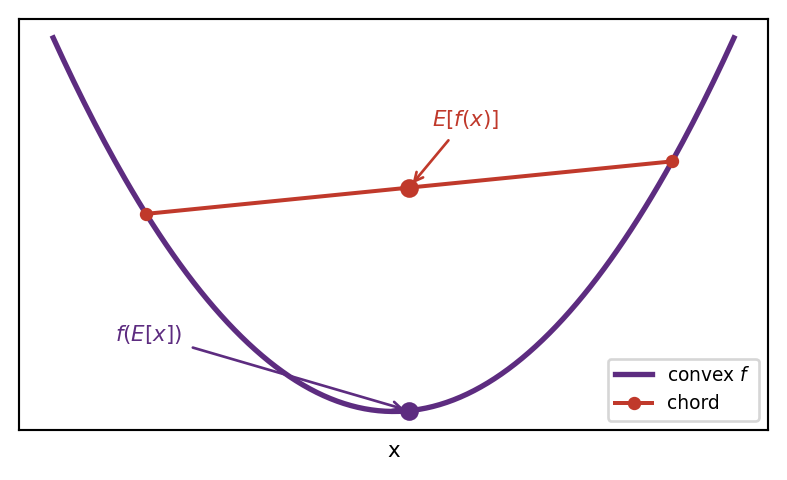
Since \(-\ln\) is convex, Jensen (previous slide) guarantees \(\mathrm{KL}\ge 0\) — it acts like a “distance” to the truth (though it is not symmetric).
\(\mathrm{KL}(p\|q)\neq\mathrm{KL}(q\|p)\) — direction matters. This asymmetry shapes how VAEs behave (later).
How much does one variable tell you about another?
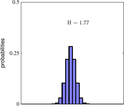
Two more quantities, both built from entropy:
Conditional entropy — uncertainty left in \(y\)after seeing \(x\): \[ \mathrm H[y\given x] = -\sum_{x,y} p(x,y)\,\ln p(y\given x) \] with the chain rule \(\;\mathrm H[x,y]=\mathrm H[x]+\mathrm H[y\given x]\).
Mutual information — how much \(x\)reduces uncertainty about \(y\): \[ \mathrm I[x,y] = \mathrm H[y]-\mathrm H[y\given x] = \mathrm{KL}\big(p(x,y)\,\|\,p(x)p(y)\big) \ge 0 \]\(\mathrm I=0 \iff x,y\)independent.
Back to rain & umbrella: they were dependent, so \(\mathrm I[\text{rain},\text{umb}]\approx 0.09\) nats \(>0\) — knowing one genuinely lowers uncertainty about the other. Representation learning (L11) trains features by maximizing mutual information with the input (contrastive / InfoNCE).
Bishop §2.5.6–2.5.7
Continuous distributions (preview)
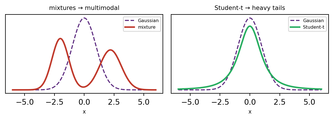
We’ve met the Gaussian — the workhorse. A few more continuous densities show up later:
Mixture of Gaussians\(\sum_k \pi_k\,\mathcal N(x\given\vmu_k,\boldsymbol\Sigma_k)\) — multimodal data & clustering (L19, EM)
Student-t / Laplace — heavier tails → robust to outliers
Beta / Dirichlet — densities over probabilities themselves (Bayesian priors)
Bishop §3.2–3.5. The Gaussian, Beta and Dirichlet — with Bernoulli/Categorical (next) — belong to the exponential family, a unifying umbrella; mixtures and Student-t are not (notable exceptions).
Discrete distributions (preview)
For the classification lecture we’ll need distributions over categories:
Categorical — one of \(K\) classes: \[ p(\vt\given\boldsymbol\mu) = \prod_{k=1}^{K}\mu_k^{\,t_k} \]
Bishop §3.1 — these give the cross-entropy loss in classification (L3), the way the Gaussian gives sum-of-squares in regression (L2).
Summary
Two rules — sum & product — generate all of probability; Bayes reverses conditionals
Densities: area (an integral), not height, is probability; transforms rescale by the Jacobian
Gaussian + maximum likelihood — our default noise model and how we fit parameters from data
Information theory: entropy, KL (≥0 by Jensen), cross-entropy, mutual information — the language of loss & representation learning
These are the tools the whole course runs on: MLE → squared error (L2), cross-entropy → classification (L3), KL → VAEs & diffusion (L12). Keep this deck as your reference.
📌 Read before next class
Lecture 2 — Linear Regression. We turn maximum likelihood under Gaussian noise into the squared-error loss and its closed-form least-squares solution.