Lecture 5 — Deep Neural Networks

Deep Learning · Session 5

Kasemsit Teeyapan

Department of Computer Engineering, Chiang Mai University

Today

Why fixed basis functions break down in high dimensions
The multilayer perceptron: learning the features \(\boldsymbol{\phi}\) instead of choosing them
Activation functions — and why nonlinearity is essential
Universal approximation — and why we still go deep
The output & loss are unchanged — only \(\boldsymbol{\phi}\) is now learned

Reference: Bishop & Bishop (2024), Chapter 6 — Deep Neural Networks

Recap → the big leap

So far (L2–L3): \[ y(\vx,\vw) = \vw^{\mathsf T}\boldsymbol{\phi}(\vx) \]

\(\boldsymbol{\phi}\) fixed by hand (polynomial, Gaussian…)
linear in \(\vw\) → closed form
L3: a good \(\boldsymbol{\phi}\) makes classes separable — but we picked it

Today: \[ \boldsymbol{\phi}(\vx) = h(\mathbf W^{(1)}\vx) \;\;\text{— learned} \]

the features adapt to the data
no closed form → gradient descent (next lectures)

The leap from classical ML to deep learning: stop choosing features, start learning them

Part 1 · Why Not Just Fix the Basis?

The curse of dimensionality

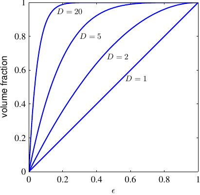
To tile input space with fixed basis functions, the number needed grows exponentially with dimension \(D\).

images: \(D\) = millions of pixels
a grid of fixed bumps is hopeless

Split each input axis into just 10 bins. How many fixed basis bumps does it take to tile a \(D=10\) space — thousands, millions, or more?

Fixed bases can’t scale to high-dimensional data — we need bases that focus where the data actually is.

\(b=10\) bins per axis \(\Rightarrow b^{D}\) bumps. \(D{=}1\!:10\), \(D{=}2\!:100\), \(D{=}3\!:1000\), \(D{=}10\!:\mathbf{10^{10}}\) (ten billion). A tiny \(100{\times}100\) image (\(D{=}10^4\)) would need \(10^{10000}\) — far more than the atoms in the universe. Did your guess reach ten billion?

Source: Bishop & Bishop (2024), Deep Learning, Fig 6.4 — most volume of a high-D region sits near its surface

curse of dimensionality: จำนวน fixed basis ที่ต้องใช้ “ปูพื้นที่” โตแบบ exponential ตามมิติ D ภาพมี D เป็นล้าน → grid ของ bump คงที่เป็นไปไม่ได้ รูป: ปริมาตรเกือบทั้งหมดของก้อนมิติสูงอยู่ใกล้ผิว (intuition แปลก ๆ ของ high-D) เฉลย predict/worked: 10 bins ต่อแกน → 10^D; D=10 ได้ 10^10 = หมื่นล้าน, ภาพ 100×100 (D=10^4) → 10^10000 มากกว่าอะตอมในจักรวาล ย้ำว่าแค่ ~3 bins/แกนก็สิ้นหวังแล้ว → ต้องมี basis ที่โฟกัสตรงที่ข้อมูลอยู่จริง ~2 นาที

But real data lives on a manifold

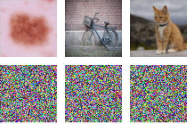
real images (top) occupy a tiny sliver of pixel space
random pixels (bottom) are never natural images
the data sits on a low-dimensional manifold

So: don’t cover all of space — learn features that follow the data manifold. That is what hidden layers do.

Source: Bishop & Bishop (2024), Deep Learning, Fig 6.8

Part 2 · The Multilayer Perceptron

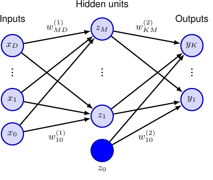
A two-layer network

Forward propagation: \[ \mathbf z = h\!\big(\mathbf W^{(1)}\vx + \mathbf b^{(1)}\big) \] \[ \mathbf y = \mathbf W^{(2)}\mathbf z + \mathbf b^{(2)} \]

\(\mathbf z\) = learned features \(\boldsymbol{\phi}(\vx)\)
two layers of weights \(\mathbf W^{(1)}, \mathbf W^{(2)}\)
\(h\) = nonlinear activation

This is exactly \(y=\vw^{\mathsf T}\boldsymbol{\phi}(\vx)\) from Lecture 2 — but the hidden layer \(\boldsymbol{\phi}(\vx)=h(\mathbf W^{(1)}\vx)\) is now learned.

Feed \(\vx=(1,2)\) into a hidden unit computing \(\text{ReLU}(1\!\cdot\!x_1 - 1\!\cdot\!x_2)\). Is that unit active (positive output) or dead (zero) for this input?

Source: Bishop & Bishop (2024), Deep Learning, Fig 6.9

Worked: one forward pass

A 2-input → 2-hidden → 1-output net, \(h=\text{ReLU}\): \[ \mathbf W^{(1)}=\begin{bmatrix}1&-1\\[-1pt]0&2\end{bmatrix},\;\; \mathbf b^{(1)}=\begin{bmatrix}0\\[-1pt]-1\end{bmatrix},\;\; \mathbf W^{(2)}=\begin{bmatrix}2&1\end{bmatrix},\;\; b^{(2)}=0,\;\; \vx=\begin{bmatrix}1\\[-1pt]2\end{bmatrix} \]

① Pre-activations \(\;\mathbf a=\mathbf W^{(1)}\vx+\mathbf b^{(1)}=\begin{bmatrix}1\!-\!2+0\\ 0\!+\!4-1\end{bmatrix}=\begin{bmatrix}-1\\ 3\end{bmatrix}\)

② Hidden \(\;\mathbf z=\text{ReLU}(\mathbf a)=\begin{bmatrix}0\\ 3\end{bmatrix}\) — unit 1 is dead (matches the prediction)

③ Output \(\;y=\mathbf W^{(2)}\mathbf z+b^{(2)}=2(0)+1(3)=\mathbf 3\)

The dead unit contributes nothing to \(y\). A ReLU net partitions inputs by which units fire — the heart of the “folding” we’ll see in Part 4.

Your turn: a different input

Same network as the worked example (\(\mathbf W^{(1)},\mathbf b^{(1)},\mathbf W^{(2)}\) unchanged). Now feed \(\vx=(3,1)\).

Compute the pre-activations \(\mathbf a\), the hidden vector \(\mathbf z\), and the output \(y\). Is hidden unit 1 still dead?

Why the nonlinearity matters

Without \(h\), stacking layers collapses:

\[ \mathbf W^{(2)}\big(\mathbf W^{(1)}\vx\big) = \underbrace{\big(\mathbf W^{(2)}\mathbf W^{(1)}\big)}_{\text{just another matrix}}\vx \quad=\text{ a single linear layer!}\]

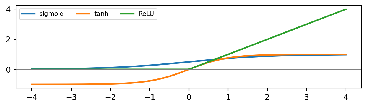
import numpy as np, matplotlib.pyplot as plt
a = np.linspace(-4, 4, 200)
plt.figure(figsize=(6.6, 2.0))
for name, f in [("sigmoid", 1/(1+np.exp(-a))), ("tanh", np.tanh(a)), ("ReLU", np.maximum(0, a))]:
    plt.plot(a, f, label=name, lw=2)
plt.axhline(0, color="grey", lw=.5); plt.legend(fontsize=8, ncol=3); plt.tight_layout(); plt.show()

The activation \(h\) is what makes depth meaningful · ReLU \(=\max(0,a)\) is the modern default (no vanishing-gradient saturation)

Worked: collapse, and how ReLU saves it

Stack two linear layers \(\mathbf W^{(2)}\big(\mathbf W^{(1)}\vx\big)\) with no activation. Can a single matrix \(\mathbf M\) reproduce them exactly for every \(\vx\)?

Take \(\mathbf W^{(1)}=\begin{bmatrix}1&2\\[-1pt]0&1\end{bmatrix},\;\; \mathbf W^{(2)}=\begin{bmatrix}1&0\\[-1pt]1&1\end{bmatrix}\).

No activation \(\Rightarrow\) collapse: \(\;\mathbf M=\mathbf W^{(2)}\mathbf W^{(1)}=\begin{bmatrix}1&2\\ 1&3\end{bmatrix}\). Check \(\vx=(1,1)\): two layers give \((3,4)\); \(\mathbf M\vx=(3,4)\) ✓ — one matrix suffices.

Insert ReLU between them, \(\vx=(1,-1)\): \(\;\mathbf W^{(1)}\vx=(-1,-1)\xrightarrow{\text{ReLU}}(0,0)\Rightarrow\) output \((0,0)\). But \(\mathbf M\vx=(-1,-2)\) — no linear map gives \((0,0)\) here. Nonlinearity is what stops the collapse.

Part 3 · Universal Approximation

One hidden layer is already universal

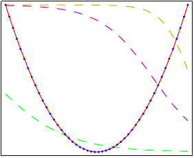
Theorem (Cybenko 1989; Hornik 1991): a network with one hidden layer and enough units can approximate any continuous function on a bounded region to arbitrary accuracy.

dashed = individual hidden units
their weighted sum (red) fits the target (blue)

“Can approximate” = existence, not a recipe — it may need exponentially many units, and says nothing about learning them.

Approximation is built from localized bumps. How few ReLU units does it take to make one triangular bump — rising, then back to zero?

Source: Bishop & Bishop (2024), Deep Learning, Fig 6.10 — a 2-layer net fitting \(x^2\)

Universal approximation (Cybenko 1989, Hornik 1991): net ชั้นซ่อนเดียว + หน่วยพอ → ประมาณฟังก์ชันต่อเนื่องใด ๆ บนช่วงจำกัดได้แม่นเท่าใดก็ได้ รูป: เส้นประ=หน่วยซ่อนแต่ละตัว, ผลรวม(แดง)=fit เป้าหมาย(น้ำเงิน) ข้อควรระวัง (สำคัญ!): “ประมาณได้” = มีอยู่จริง ไม่ใช่วิธีหา + อาจต้องใช้หน่วย exponential + ไม่ได้บอกว่าจะ “เรียน” เจอไหม → ปูเหตุผลทำไมต้องลึก predict: สร้าง bump สามเหลี่ยมจาก ReLU ใช้กี่ตัว? (เฉลย 3 ตัว — สไลด์ถัดไป) ~2.5 นาที

Worked: a bump from three ReLUs

\[ g(x)=\text{ReLU}(x)\;-\;2\,\text{ReLU}(x-1)\;+\;\text{ReLU}(x-2) \]

Evaluate piece by piece: \(g(0.5)=0.5\) (rising) \(\to g(1)=\mathbf 1\) (peak) \(\to g(1.5)=0.5\) (falling) \(\to g(3)=0\). A triangle on \([0,2]\), peak \(1\) at \(x=1\) — from just 3 ReLUs. Sum many shifted/scaled bumps \(\Rightarrow\) any continuous function. That is universal approximation, by construction — and why a sum of ReLUs is piecewise-linear (the closing puzzle).

Using two ReLUs, build a step that rises from \(0\) to \(1\) as \(x\) goes from \(2\) to \(4\). Evaluate it at \(x=3\).

worked: g(x)=ReLU(x)−2ReLU(x−1)+ReLU(x−2) → ค่อย ๆ ไล่: x=0.5→0.5, x=1→1 (ยอด), x=1.5→0.5, x=3→0 = สามเหลี่ยมบน [0,2] ยอด 1 จาก ReLU แค่ 3 ตัว รวม bump หลาย ๆ อัน (เลื่อน/ปรับสเกล) → ประมาณฟังก์ชันต่อเนื่องใด ๆ = universal approximation แบบสร้างจริง และอธิบายว่าทำไมผลรวม ReLU เป็น piecewise-linear (โยงโจทย์ท้ายคาบ) เฉลย solo (อย่าเขียนบนสไลด์): g(x)=½[ReLU(x−2)−ReLU(x−4)] → x<2:0, x=3: ½(1−0)=0.5, x≥4: ½(2−0)… = ½[(x−2)−(x−4)]=½·2=1 → step สูง 1 ระหว่าง 2 ถึง 4, ที่ x=3 ได้ 0.5 ให้เวลา ~2 นาที ~3 นาที

🔬 Demo: build a function from ReLUs

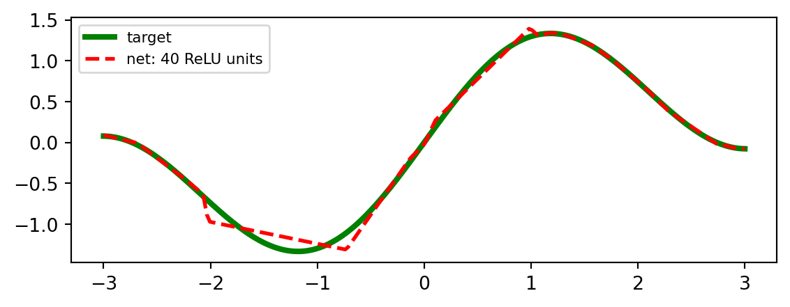
import numpy as np, matplotlib.pyplot as plt
rng = np.random.default_rng(0)
x = np.linspace(-3, 3, 200); target = np.sin(1.5*x) + 0.3*x
M = 40                                        # hidden ReLU units with random weights
W = rng.normal(0, 1.5, M); b = rng.normal(0, 3, M)
H = np.maximum(0, np.outer(x, W) + b)         # hidden features  z = ReLU(Wx+b)
v = np.linalg.lstsq(H, target, rcond=None)[0] # learn only the output weights
plt.figure(figsize=(6, 2.4))
plt.plot(x, target, "g", lw=3, label="target")
plt.plot(x, H @ v, "r--", lw=2, label="net: 40 ReLU units")
plt.legend(fontsize=8); plt.tight_layout(); plt.show()

40 hidden units already trace the target — a hidden layer is a flexible, learnable basis.

Part 4 · Why Go Deep?

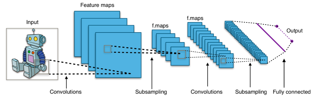
Depth builds a hierarchy of features

one wide layer can approximate — but depth is exponentially more efficient for compositional functions
each layer reuses the previous layer’s features (edges → parts → objects)
distributed representations: features combine, so capacity grows fast

Depth turns “approximate anything” (existence) into “represent structure efficiently” (practice)

Source: Wikimedia Commons — Typical CNN by Aphex34, CC BY-SA 4.0 · depth ≈ composition (Bishop §6.3)

ทำไมต้องลึก ไม่ใช่แค่กว้าง: (1) ชั้นกว้างชั้นเดียวประมาณได้ แต่ depth มีประสิทธิภาพกว่าแบบ exponential สำหรับฟังก์ชันเชิงประกอบ (2) แต่ละชั้นนำ feature ชั้นก่อนมาประกอบใหม่ (ขอบ→ชิ้นส่วน→วัตถุ) (3) distributed representation: feature ผสมกันได้ → capacity โตเร็ว เชื่อม L0 (representation learning) ย้ำ pillar: depth เปลี่ยน “ประมาณได้” เป็น “แทนโครงสร้างได้อย่างมีประสิทธิภาพ” ~2.5 นาที

Depth vs width: an exponential gap

Universal approximation says one wide layer suffices — but how wide?

For some functions, a deep net needs only \(O(d)\) units where a shallow one needs \(O(2^d)\).

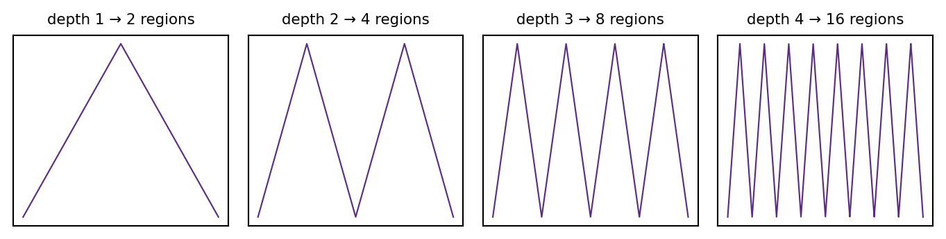
Why: each layer can fold its input. Composing \(d\) folds creates \(2^d\) linear regions — exponential structure from linear depth.

Pillar: depth buys representational efficiency. The same function can be exponentially cheaper to express deep than wide (Telgarsky 2016; Montúfar et al. 2014).

A tent map = 1 fold = 2 ReLU units, and each fold doubles the linear pieces. Compose 4 such layers (8 units total). How many linear “teeth” — 8, 16, or 32?

depth vs width — เติมความลึกเชิงทฤษฎีให้ “why deep”: universal approximation บอกชั้นเดียวพอ “แต่กว้างแค่ไหน?” คำตอบ: บางฟังก์ชัน deep ใช้ O(d) หน่วย ขณะ shallow ต้อง O(2^d) เหตุผลเชิงเรขาคณิต: แต่ละชั้น “พับ” (fold) input ได้ พับ d ครั้ง → 2^d ช่วงเชิงเส้น = โครงสร้าง exponential จากความลึกเชิงเส้น ย้ำ pillar: depth ซื้อ “representational efficiency” — ฟังก์ชันเดียวกันแสดงด้วย deep ถูกกว่า wide แบบ exponential (Telgarsky 2016, Montúfar 2014) นี่คือคำตอบเชิงทฤษฎีว่าทำไมลึกถึงดีกว่ากว้าง เดี๋ยว demo ให้เห็นการพับ ~2.5 นาที

🔬 Demo: each layer folds the input

import numpy as np, matplotlib.pyplot as plt
tent = lambda x: np.where(x < 0.5, 2*x, 2*(1-x))      # one fold = 2 ReLU units
x = np.linspace(0, 1, 4000)
fig, ax = plt.subplots(1, 4, figsize=(7.2, 1.9), sharey=True)
for a, d in zip(ax, [1, 2, 3, 4]):
    y = x.copy()
    for _ in range(d): y = tent(y)                     # compose d folds (a depth-d net)
    a.plot(x, y, lw=0.8, color="#5d2c80")
    a.set_title(f"depth {d} → {2**d} regions", fontsize=8); a.set_xticks([]); a.set_yticks([])
plt.tight_layout(); plt.show()

Depth 4 → \(2^4=\mathbf{16}\) teeth from 8 units. Did your guess match?

Those 16 teeth take ~1 unit per tooth in a shallow (1-hidden-layer) net. Compare the unit count: shallow vs this depth-4 net. Then redo it for 1024 teeth.

demo: tent map (พับครั้งเดียว = 2 ReLU) ประกอบกัน d ชั้น = net ลึก d ชั้น ผล: depth 1→2 ฟัน, 2→4, 3→8, 4→16 ฟัน — จำนวนช่วงเชิงเส้นโตเป็น 2^d ขณะที่จำนวนหน่วยโตแค่ ~2d ชี้: ถ้าจะให้ shallow net (ชั้นเดียว) สร้าง 16 ฟันต้องใช้ ~16 หน่วย แต่ deep ใช้แค่ ~8 หน่วย (4 ชั้น × 2) — ยิ่ง d โตช่องว่างยิ่ง exponential นี่คือเหตุผลเชิงประจักษ์ว่าทำไมเครือข่ายลึกแสดงฟังก์ชันซับซ้อนได้ด้วยพารามิเตอร์น้อยกว่า เชื่อม compositionality ของข้อมูลจริง (ภาพ/ภาษาเป็นลำดับชั้น) เฉลย solo: 16 ฟัน → shallow ~16 หน่วย vs deep 8 หน่วย (4×2); 1024 ฟัน → shallow ~1024 หน่วย vs deep ~20 หน่วย (10 ชั้น × 2) = ช่องว่าง exponential ~2 นาที

Representation learning

The hidden layers discover the features — exactly the “learn from data” idea from Lecture 0.

early layers: generic, low-level (edges, textures)
later layers: task-specific, high-level (object parts)
these learned features transfer to new tasks (pretraining → fine-tuning)

This is why melanoma & AlphaFold worked: no hand-designed features — the network learned \(\boldsymbol{\phi}\).

Part 5 · Same Loss, Learned Features

The output and loss are unchanged

The network just replaces fixed \(\boldsymbol{\phi}\) with a learned one. The head and loss are exactly Lectures 2–3:

Regression → linear output, squared error \[ E=\tfrac12\textstyle\sum_n\{y_n-t_n\}^2 \]

Classification → softmax output, cross-entropy \[ E=-\textstyle\sum_n\sum_k t_{nk}\ln y_{nk} \]

Same maximum-likelihood losses — the only new thing is that \(\boldsymbol{\phi}\) has parameters too, so there is no closed form

To train \(\mathbf W^{(1)}, \mathbf W^{(2)}\) we need the gradient of \(E\) — that is backpropagation (next lectures).

Summary

Fixed bases fail in high-D (curse of dimensionality); real data lies on a manifold
An MLP learns the features: \(\boldsymbol{\phi}(\vx)=h(\mathbf W^{(1)}\vx)\) — the nonlinearity \(h\) makes depth meaningful
Universal approximation: one hidden layer suffices in principle; depth makes it efficient
Output & loss are still MLE (squared error / cross-entropy) — but now there’s no closed form → backprop

Something to think about: a 2-layer net uses ReLU hidden units but a linear output. Is the overall function piecewise-linear or smooth? (Hint: a sum of ReLUs.)

📌 Read before next class

Bishop & Bishop (2024), Chapter 7 — Gradient Descent

How do we actually minimize \(E(\vw)\) when there is no closed form? Gradient descent, SGD, momentum, and learning-rate schedules.

Figures from Bishop & Bishop, Deep Learning: Foundations and Concepts (2024), Chapter 6 — https://www.bishopbook.com/