\( \newcommand{\vw}{\mathbf{w}} \newcommand{\vx}{\mathbf{x}} \newcommand{\vt}{\mathbf{t}} \newcommand{\vy}{\mathbf{y}} \newcommand{\vz}{\mathbf{z}} \newcommand{\vq}{\mathbf{q}} \newcommand{\vk}{\mathbf{k}} \newcommand{\vv}{\mathbf{v}} \newcommand{\vc}{\mathbf{c}} \newcommand{\vp}{\mathbf{p}} \newcommand{\vh}{\mathbf{h}} \newcommand{\vmu}{\boldsymbol{\mu}} \newcommand{\vsigma}{\boldsymbol{\sigma}} \newcommand{\vepsilon}{\boldsymbol{\epsilon}} \newcommand{\R}{\mathbb{R}} \newcommand{\E}{\mathbb{E}} \newcommand{\norm}[1]{\lVert #1 \rVert} \newcommand{\given}{\,\vert\,} \)

Lecture 20 — Sampling: MCMC & Langevin

Deep Learning · Monte Carlo, Metropolis–Hastings, Langevin

Kasemsit Teeyapan

Department of Computer Engineering, Chiang Mai University

Today

  1. Why sample — intractable integrals become Monte Carlo averages
  2. Rejection sampling — simple, but wasteful in high dimensions
  3. MCMC & Metropolis–Hastings — a random walk that converges to \(p(\vx)\)
  4. Langevin dynamics — sampling with the gradient \(\nabla\ln p(\vx)\)
  5. The bridge: score-based diffusion (L12) = learned Langevin

Reference: Bishop & Bishop (2024), Chapter 14Sampling

Why sample? — estimate π with darts

Throw \(S\) random darts at a unit square. The fraction that land inside the quarter-circle (\(x^2+y^2<1\)), times 4, \(\approx\pi\):

\[\pi \approx 4\cdot\frac{\#\{x^2+y^2<1\}}{S}\]

\(S=100\) → rough; \(S=10^6\)\(3.14\ldots\). We just computed an integral (an area) by averaging samples.

In general, any expectation is a sample average: \[\E_{p}[f(\vx)]=\int f(\vx)\,p(\vx)\,d\vx \approx \frac1S\sum_{s=1}^{S} f(\vx_s)\]

unbiased; error \(\sim 1/\sqrt S\), independent of dimension.

But how to draw \(\vx_s\sim p\) when \(p\) is high-D and known only up to a constant?

Rejection sampling

Draw from an easy \(q(\vx)\) that covers \(p\) (\(Mq(\vx)\ge \tilde p(\vx)\)), then keep \(\vx\) with probability \(\tilde p(\vx)/Mq(\vx)\).

  • correct, and needs only unnormalized \(\tilde p\)
  • but the accept rate \(\propto 1/M\) collapses in high dimensions → hopeless for big models

The curse of dimensionality (L5) strikes again: a proposal that covers \(p\) in 100-D almost never lands in the right place. We need a method that walks toward high-probability regions.

MCMC & Metropolis–Hastings

Build a Markov chain whose stationary distribution is \(p\). From \(\vx\), propose \(\vx'\sim q(\vx'\given\vx)\) and accept with probability

\[A=\min\!\Big(1,\ \frac{\tilde p(\vx')\,q(\vx\given\vx')}{\tilde p(\vx)\,q(\vx'\given\vx)}\Big)\]

  • symmetric \(q\)\(A=\min(1,\,\tilde p(\vx')/\tilde p(\vx))\)
  • uphill always accepted; downhill sometimes → explores while favoring high \(p\)

Pillar: detailed balance guarantees the chain converges to \(p\) — using only ratios, so the unknown normalizing constant cancels. That’s why MCMC works for posteriors.

Langevin dynamics

Use the gradient to walk uphill in \(\ln p\), plus noise to keep exploring:

\[\vx_{t+1}=\vx_t+\varepsilon\,\nabla\ln p(\vx_t)+\sqrt{2\varepsilon}\,\boldsymbol\xi,\quad \boldsymbol\xi\sim\mathcal N(0,I)\]

  • gradient ascent on \(\ln p\) + calibrated noise
  • as \(\varepsilon\to0\) the stationary distribution is exactly \(p\)
  • needs only the score \(\nabla\ln p\) — the constant cancels again

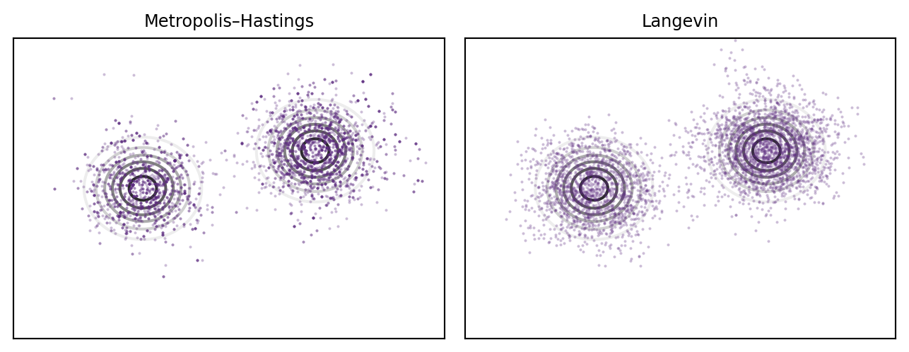
Pillar: gradient descent finds a mode; adding \(\sqrt{2\varepsilon}\) noise turns it into sampling from the whole distribution. Optimization and sampling differ by a noise term.

🔬 Demo: MCMC vs Langevin

import numpy as np, matplotlib.pyplot as plt
rng = np.random.default_rng(0); cen = np.array([[-2,0],[2,1]]); s2 = 0.7**2
def logp(x):  d=x-cen; q=-0.5*np.sum(d*d,1)/s2; m=q.max(); return m+np.log(np.exp(q-m).sum())
def score(x): d=x-cen; w=np.exp(-0.5*np.sum(d*d,1)/s2); w/=w.sum(); return -(w[:,None]*d).sum(0)/s2

x=np.zeros(2); M=[]                                            # Metropolis
for _ in range(4000):
    xp=x+rng.normal(0,0.8,2)
    if np.log(rng.random())<logp(xp)-logp(x): x=xp
    M.append(x.copy())
x=np.zeros(2); L=[]; eps=0.05                                  # Langevin
for _ in range(4000):
    x=x+eps*score(x)+np.sqrt(2*eps)*rng.normal(0,1,2); L.append(x.copy())
M,L=np.array(M[200:]),np.array(L[200:])
gx,gy=np.meshgrid(np.linspace(-5,5,120),np.linspace(-4,4,120))
Z=np.array([np.exp(logp(np.array([a,b]))) for a,b in zip(gx.ravel(),gy.ravel())]).reshape(gx.shape)
fig,ax=plt.subplots(1,2,figsize=(6.8,2.7))
for a,S,t in [(ax[0],M,"Metropolis–Hastings"),(ax[1],L,"Langevin")]:
    a.contour(gx,gy,Z,levels=6,cmap="Greys"); a.plot(S[:,0],S[:,1],".",ms=1,alpha=.3,color="#5d2c80")
    a.set_title(t,fontsize=9); a.set_xticks([]); a.set_yticks([])
plt.tight_layout(); plt.show()
The bridge: score-based diffusion

Langevin needs only the score \(\vs(\vx)=\nabla\ln p(\vx)\). For real data we don’t have \(p\) — so learn the score with a network \(\vs_\theta(\vx)\approx\nabla\ln p(\vx)\) (score matching).

Then sample by Langevin using \(\vs_\theta\).

Pillar: that is exactly a diffusion model (L12) — the reverse process is learned-score Langevin across noise levels. Sampling theory (this lecture) + a learned score = modern generative AI.

Summary

  1. Monte Carlo turns intractable integrals into sample averages (error \(\sim 1/\sqrt S\))
  2. Rejection sampling is exact but dies in high dimensions
  3. MCMC / Metropolis–Hastings walks to \(p\) using only ratios (constant cancels)
  4. Langevin = gradient of \(\ln p\) + noise; optimization + noise = sampling
  5. Score-based diffusion (L12) = Langevin with a learned score

Something to think about: Langevin and SGD (L6) have the same shape — a gradient step plus noise. SGD’s noise comes from mini-batches. What would it mean to view SGD as sampling rather than optimizing?

📌 Connections

Sampling completes the generative picture: EM (L19) and VAEs (L12) approximate the posterior; MCMC/Langevin sample it; diffusion (L12) learns the score and samples by Langevin.

References: Metropolis et al. (1953); Hastings (1970); Welling & Teh, Bayesian Learning via Stochastic Gradient Langevin Dynamics (2011); Song & Ermon, Score-Based Generative Modeling (2019). Figures/derivations from Bishop & Bishop (2024), Ch 14 — https://www.bishopbook.com/

⌂ Home